By: Hao Chang Electrical and Luigi Vanfretti, Computer and Systems Engineering – Rensselaer Polytechnic Institute Troy, NY
This article summarizes the results of a project that we – Rensselaer Polytechnic Institute (RPI) – conducted in collaboration with Smarter Grid Solutions to test smart inverter functionalities, which is supported by the New York State Energy and Research Development Authority (NYSERDA). The project established a Power Hardware-in-the-Loop (PHIL) experimental facility for smart inverter testing, with the goal of verifying its compliance with the IEEE 1547.1- 2020 standard, for interconnecting distributed energy resources (DER) with electrical power systems (EPSs). This setup was successfully used to test the functionality of the SMA inverter in different operating conditions and control modes. The six experiments documented in the original paper include the testing of the inverter operating in control modes: constant power factor, constant reactive power, voltage-var, voltage watt, voltage ride through and return to service. In this article we will detail only the “Constant Power Factor Mode” experiment.
PHIL LABORATORY EXPERIMENTAL FACILITY
OPAL-RT OP1400 power amplifier
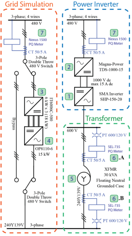
The OP1400 power amplifier labeled 4 in Figure 1 is an essential component of the experimental platform, as it emulates the power grid to which the inverter is connected. To control and monitor the amplifier, a user interface (UI) has been implemented; see Fig. 2. The UI serves as the control panel for the OP1400 power amplifier and is executed using a real-time simulator. This interface is critical in ensuring the successful operation of the experimental platform during the testing experiments, as it allows the user to adjust parameters and observe the system’s behavior in real-time. In Figure 2, enclosed in red squares and numbered, are the different experiment control and monitoring functions used to carry out the tests:
- Automated RMS Voltage Set-point Adjustment
- Voltage Set-point Adjustment
- Voltage Slew-rate Limiter
- Voltage Set-point Display
- RMS Voltage and Current for Each Phase (Monitoring)
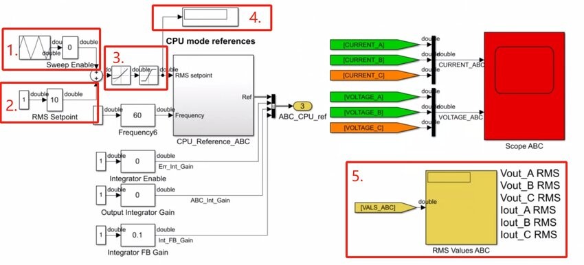
In the following experiments, the 3-Phase RMS Voltage Set-Point is used to control the input voltage for the inverter to conduct High/Low voltage ride-through tests. The Automated RMS Voltage Set-Point Adjustment is used to automatically change the input voltage for the inverter to obtain the characteristic graphs of Volt-Watt and Volt-Var control mode operation. The Slew-Rate limiter is used to limit the impact of the autotransformer inrush current. This was necessary since during the coupling of the experimental platform it was observed that in experiments when the voltage was changed too quickly, the power amplifier’s protections would trip because of the autotransformer’s inrush current. The Saturation Limiter avoids user input errors that exceed the amplifier and inverter voltage limits. The voltage saturates at 160 Vrms L-N. Therefore, the voltage can reach 692 VLL on the high side of the autotransformer, which is sufficient for all testing procedures within the scope of the experimental facility.
DC power supply
The DC power supply labeled as number 2 shown in Fig. 1 is used to emulate a Photovoltaic (PV) cell working under different conditions. The Photovoltaic Power Profile Emulation (PPPE) software automatically calculates the solar array voltage and current profiles based on user-defined parameters. Since the experiments do not require a change on the DC side and the maximum active power output of the inverter is set to 3 kW. Meanwhile, the profile in box 1 is sent to the DC power supply to have a maximum of 7.2 kW, which allows the DC supply to operate following the characteristic of the emulated PV panel. This power profile is used in all experiments.
SMA inverter
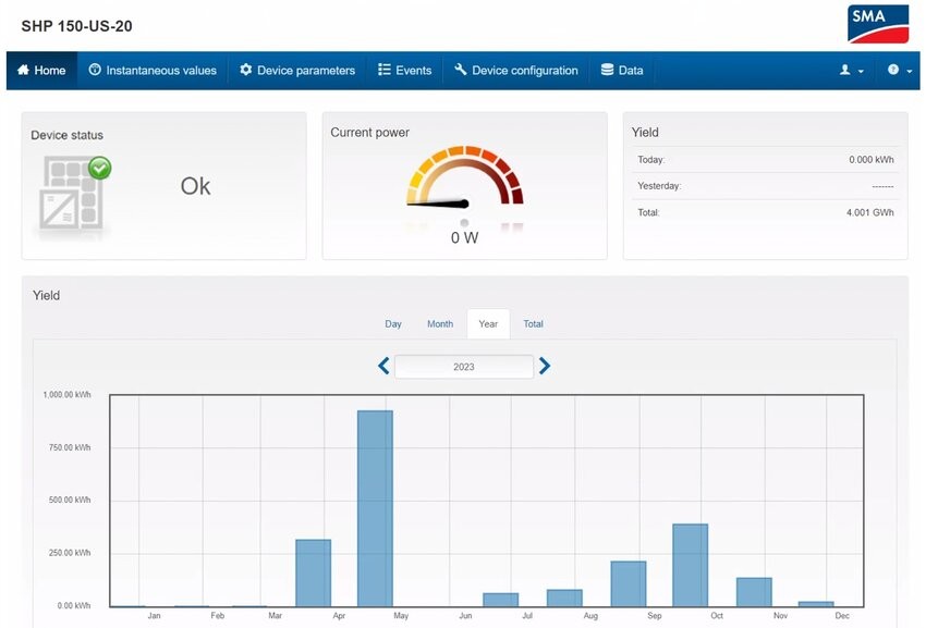
The SMA inverter is the EUT (equipment under test) for all tests carried out and documented next. The inverter is configured through its embedded server user interface, shown in Figure 3. In the UI’s main screen (i.e., the Web Server’s home page), the current output power and device status are displayed. The “Device Parameters” tab is where the configuration and settings for the inverter are displayed and can be modified. In the following experiments, the detailed settings are all displayed and configured through this tab.
Experiment – constant power factor mode
Understanding how an inverter interacts with the grid under constant power factor conditions is crucial for the integration of renewable energy sources, as it affects the stability and efficiency of the grid. In the following test, the constant power factor (pf) mode of the inverter will be tested with a 0.95 lagging power factor. From the UI, the power factor is set to be constant at 0.95. Measurement data were recorded after the inverter finished adjusting the output power (i.e., when it reached a “steady state”). These recordings are used to verify whether the inverter is outputting and maintaining the desired active and reactive power.
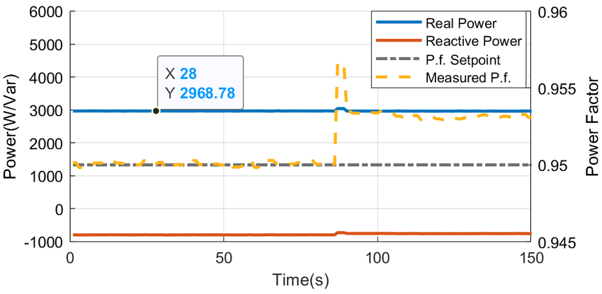
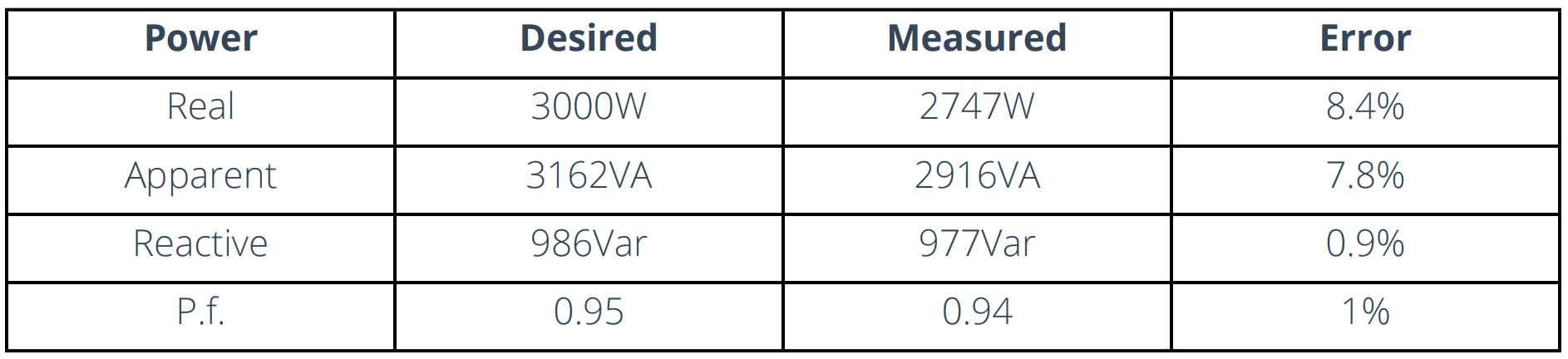
Figure 4 shows the inverter generating 3 kW and the power factor is 0.95, as expected. Since the SMA inverter is capable of generating 150 kW, 30.67 W of error is within tolerance. The oscilloscope is used to verify the lag angle. From the measurement, the time lag is 827 microseconds. In terms of angle, this corresponds to Φ = 17.8º. The desired angle is Φ = 18.2º. The measured lag angle is close to the desired angle. Noting that the waveforms are slightly distorted, the angle error can be attributed to instrumentation issues. However, the error is low and within tolerance. The experiment is repeated for an Overexcited (Leading) power factor of 0.95, and the results are shown in Table I, with similar results as in the previous test.
Table 1 – 0.95 Leading Constant Power Factor Test Results