Motor emulation on a PHIL bench for traction inverter validation
Automotive
10 / 31 / 2026

Key Takeaways
- Motor emulation lets a traction inverter run at full voltage and current against a modelled machine, so validation starts before the first prototype motor exists.
- Bench results depend on loop delay, power stage bandwidth and the quality of the machine model, which makes model data and version records part of the test evidence.
- Broad coverage and fault campaigns belong on the emulator, with a narrow set of operating points confirmed on a physical machine for correlation.
A traction inverter validated against an emulated motor at full power will meet every rotor position, torque level and fault it can face on the road before a prototype machine exists.
Programs can’t wait for that prototype. United States buyers have taken delivery of more than 8.5 million plug-in vehicles since 2010, and each one carries at least one inverter that had to be proven at power. A dynamometer spins one physical machine at a time, so your test coverage is tied to the hardware bolted to the bed. Motor emulation removes that tie.
The stronger position is to treat the modelled machine as the primary load for traction inverter testing and keep the physical motor for final confirmation. A model can be set to any speed, any torque and any fault within seconds, and it repeats the same condition tomorrow. That’s what turns inverter validation from a schedule of available hardware into a plan you control.
What motor emulation means for a traction inverter under test
Motor emulation replaces the physical machine with power electronics that behave like its windings. Your inverter connects its three phase outputs to the emulator, switches at full voltage and current, and sees the back electromotive force, inductance and rotor position signals a spinning motor would produce. Nothing rotates.
“Motor emulation replaces the physical machine with power electronics that behave like its windings.”
Picture an inverter built for a 200 kW drive unit whose motor is still in tooling. With an emulator on the phase terminals, the controls team runs current loops, field weakening and torque ramps at rated bus voltage months ahead of the first machine. Gate drivers, current sensors and busbars all carry real current while it happens.
This differs from signal level hardware in the loop, where only the controller board is tested and the power stage is simulated. Emulation at power exercises the whole inverter as a finished product. It’s how you test a traction inverter at power before the motor arrives.
How a PHIL bench reproduces rotor position at power
A power hardware in the loop (PHIL) bench runs a machine model on a real-time simulator and uses a power stage to impose the model’s terminal behaviour on your inverter. The simulator measures phase voltages, solves the motor equations, and commands the currents the modelled machine would draw, while it synthesizes the resolver or encoder signals your controller reads.
Speed sets the difficulty. An 8-pole machine at 18,000 rpm has an electrical frequency of 1,200 Hz, so one electrical cycle lasts about 833 microseconds, and a single microsecond of delay in the loop shifts the emulated rotor angle by roughly 0.43 electrical degrees. That’s why benches of this type run the machine model on a field-programmable gate array (FPGA) and generate the position signals from the same calculation as the phase currents. The OP1430 PHIL Prime bench from OPAL-RT follows this approach, emulating rotor position and torque at power so the inverter is validated against a modelled machine instead of a physical prototype.
How the power stage closes the loop with the model
The power stage is the part of the bench that turns model outputs into real current. It sits between the simulator and your inverter, absorbs power when the drive is motoring, returns it when the drive is regenerating, and must respond faster than the inverter’s own current loop so the emulated winding looks passive.
Consider a full torque launch followed by hard regenerative braking. On the bench, power flows from the DC source through your inverter into the emulator, then reverses within milliseconds as the model enters generation. Most benches circulate that energy back to the DC bus, so the supply only covers losses.
Circulating power has a practical consequence. A 250 kW test draws a small fraction of that from the building supply, so the lab’s electrical service stops limiting test power.
The tradeoff is bandwidth. A coupling inductance between emulator and inverter stands in for the machine winding, and its value, along with the emulator’s switching frequency and loop delay, decides which current ripple and harmonics are reproduced faithfully. Ask what the bench reproduces at your switching frequency before trusting a ripple measurement.
Which inverter behaviours an emulated motor lets you validate
An emulated motor lets you validate control performance, thermal limits, protection and efficiency across the full torque and speed map. Each operating point is a parameter set instead of a mechanical setup, so the map is swept in hours. Corner conditions such as peak torque at minimum bus voltage are held as long as the measurement needs.
Durability targets show why that coverage matters. Federal research targets in the United States hold an electric traction drive to a lifetime of 15 years or 300,000 miles, and no dynamometer schedule visits every combination of temperature, saturation and bus voltage an inverter will meet over that span. A model does. You can lower the magnet flux to represent a hot rotor, alter inductances to represent saturation, and rerun the same drive cycle.
| What you check on the inverter | What the emulated motor contributes |
| Current control stability across the speed range | Any speed and torque point is set as a parameter and held without a shaft or a cooling limit. |
| Field weakening at high speed | Back electromotive force rises with modelled speed, so the voltage limit is reached without overspeed risk. |
| Thermal margin of the power stage | Peak phase current is sustained for as long as the heat run needs, with regenerated power recirculated. |
| Position sensing and its tolerance to error | Resolver or encoder signals are generated by the model, so offset and noise are added on request. |
| Protection and safe state timing | Faults are triggered at a chosen instant and repeated identically, with no machine put at risk. |
Repeatability is the quiet benefit. A test that failed on Tuesday can be replayed on Wednesday with one parameter altered, which a thermally drifting physical machine can’t offer.
Fault cases you can run without breaking hardware

Fault testing is where a modelled machine pays back fastest. Winding faults, sensor faults and supply faults are switched into the model at a chosen electrical angle, your inverter’s protection reacts with real current flowing, and nothing is destroyed if the reaction is late.
Take a phase-to-phase short at high speed, the case nobody wants to stage on a real motor. On a physical machine it risks demagnetized magnets and a seized test stand. On the bench it’s a parameter. You can time the short at the current peak, record how quickly the inverter enters its safe state, and repeat it 20 times. A fault campaign on an emulation bench covers 5 families.
- Open-phase conditions on any motor line
- Line-to-line and turn-level short circuits in the winding
- Resolver or encoder errors such as offset, noise and signal loss
- DC link disturbances including sags, surges and loss of supply
- Loss of magnet flux representing partial demagnetization
Where emulation bench results need careful reading
Emulation results are only as good as the machine model and the bench bandwidth behind them. Electrical behaviour at the inverter terminals is reproduced well. Mechanical effects such as bearing wear, shaft resonance, gear noise and rotor heating aren’t present, and they stay with the physical test stand.
A common mistake is to parameterize the model from datasheet values and treat the outcome as final. Suppose the inductance data ignores saturation. The emulated current ripple at peak torque will read lower than the real machine produces, and a current sensor or thermal margin that looked comfortable will turn out thin.
Model data should come from finite element results or measured flux maps once they exist, and the model version belongs in every test record.
The sensible sequence is broad work on the emulator and a narrow confirmation on a real machine. A handful of operating points measured on both gives you a correlation check, and the bench then carries the regression load each time software is updated.
What a modelled machine gives your validation program
A modelled machine gives your program control over what gets tested and when. Coverage stops depending on prototype deliveries, test cell bookings and the survival of a single motor, and starts depending on how well you’ve defined the operating map, the fault list and the pass criteria.
That shift rewards discipline more than equipment. Teams that write the test matrix early, keep the machine model under version control, and rerun the full matrix on every software release find problems when they’re cheap to fix.
“Teams that treat the bench as a faster dynamometer get faster dynamometer results.”
We see the same pattern across traction programs at OPAL-RT. The inverters that reach the vehicle with few surprises were proven against a model that could be pushed to any rotor position, torque or fault, long before the first machine was built. Getting there takes patience with model data and honesty about what the bench can’t show you.

Power Electronics
10 / 30 / 2026
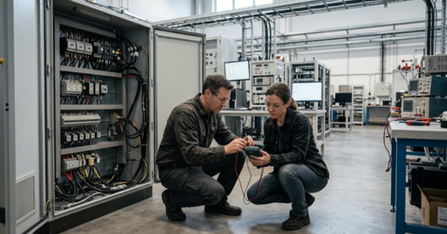
Power shelf design for high density AI racks
How a power shelf feeds a high density AI rack, which PSU topologies and efficiency targets shape it, and how GPU load steps stress its controls.
Power Electronics
10 / 29 / 2026
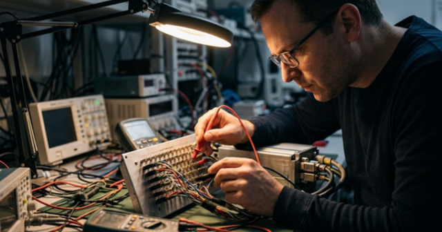
Quasi Z source inverter modeling for renewable systems
A practical look at how a quasi Z source inverter boosts and inverts in one stage, why standard models reject its boost state, and what accurate simulation and real-time testing require.
Simulation
10 / 28 / 2026
How peers troubleshoot HIL setups faster in a forum
A practical look at how searchable peer threads shorten HIL debugging, covering recurring fault types, what a good question contains and the limits of forum answers.