
Key Takeaways
- PHIL testing pays off when you treat the test bench as a power system with its own stability limits, latency budget, and protection layers.
- Fidelity comes from disciplined interface choices, deterministic timing, and measurement integrity, not from maximum model complexity or maximum power.
- Choose PHIL when power-path behavior and protection timing are the primary risks, and keep CHIL or offline simulation for earlier software and design validation.
A disciplined power hardware in the loop setup lets you test energy hardware with controlled risk.
Grid upgrades now rely heavily on power electronics, and that shift raises the cost of getting control behaviour wrong. Renewable power capacity grew by 473 GW in 2023, much of it inverter-interfaced generation that depends on fast control and protection logic. You can’t validate those interactions well with offline plots alone, and waiting for a full hardware prototype often pushes risk to the end of the schedule. Power-hardware-in-the-loop gives you a way to force the hard questions earlier, while you still have room to adjust.
The practical catch is that PHIL is not “just connect hardware to a simulator.” The outcomes depend on loop stability, measurement quality, and protection design as much as the model itself. Treat the PHIL test bench as a power system with its own dynamics, limits, and failure modes, and it will pay you back with results you can trust. Treat it as a wiring task, and it will waste time with unstable runs and misleading pass results.
Power hardware in the loop defined for energy system testing
Power hardware in the loop combines a real-time simulated power system with physical power hardware exchanging actual voltage and current. The simulator computes the network response each time step, then a power interface reproduces that response at the hardware terminals. Measurements from the hardware feed back into the simulation. The closed loop lets you validate controls and protections under power.
PHIL sits between controller-only testing and full system testing. Controller hardware-in-the-loop keeps power signals simulated, so the device under test never processes real energy. PHIL adds the power path, so you also test sensing, gating, saturation behaviour, and protection timing under realistic electrical stress. That added realism is useful when your risk is tied to power behaviour, not only control logic.
The business value comes from narrowing uncertainty around stability margins and protection coordination, not from building prettier plots. Utility-scale solar made up 53% of new U.S. electric generating capacity in 2023. A grid with more inverter-interfaced capacity will punish unstable control interactions, and PHIL is one of the few lab methods that can expose those interactions before field commissioning.
“Treat the PHIL test bench as a power system with its own dynamics, limits, and failure modes, and it will pay you back with results you can trust.”
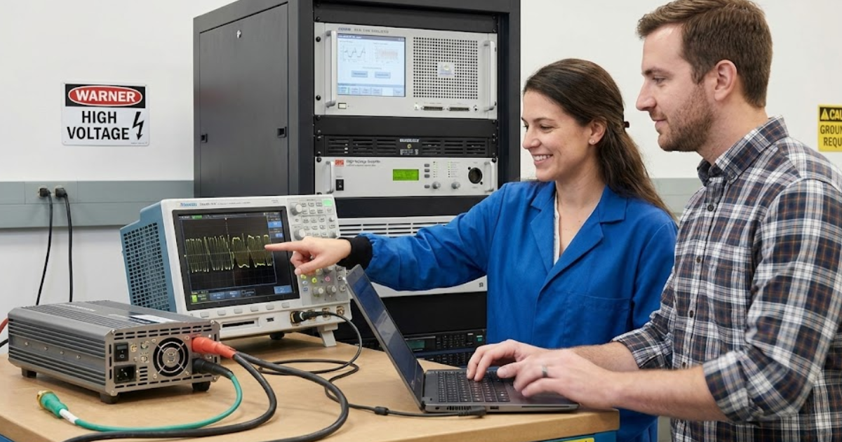
How a PHIL test bench closes the loop safely
A PHIL test bench works by running a real-time power system model, converting simulated electrical variables into physical power, and feeding measured hardware responses back into the model. The power amplifier produces the commanded voltage or current at the device terminals. Sensors capture the device’s response, then the simulator updates the network solution on the next time step. Safety comes from engineering the loop as carefully as the model.
Loop safety depends on two things you can control: energy limits and stability limits. Energy limits protect people and equipment through fast shutdown, interlocks, and fault containment. Stability limits prevent the loop from oscillating due to delay, amplifier dynamics, and measurement filtering. Both need to be designed up front, because “try it and see” can put full power into an unstable loop.
- Hardwired emergency stop that removes amplifier power independently of software
- Current and voltage limiters that act faster than the device protection
- Galvanic isolation and grounding rules that match the sensor bandwidth
- Watchdogs that trip on missed time steps and bad sensor ranges
- Fault injection paths that are bounded and repeatable for validation
Hardware, software, and interface choices that shape fidelity
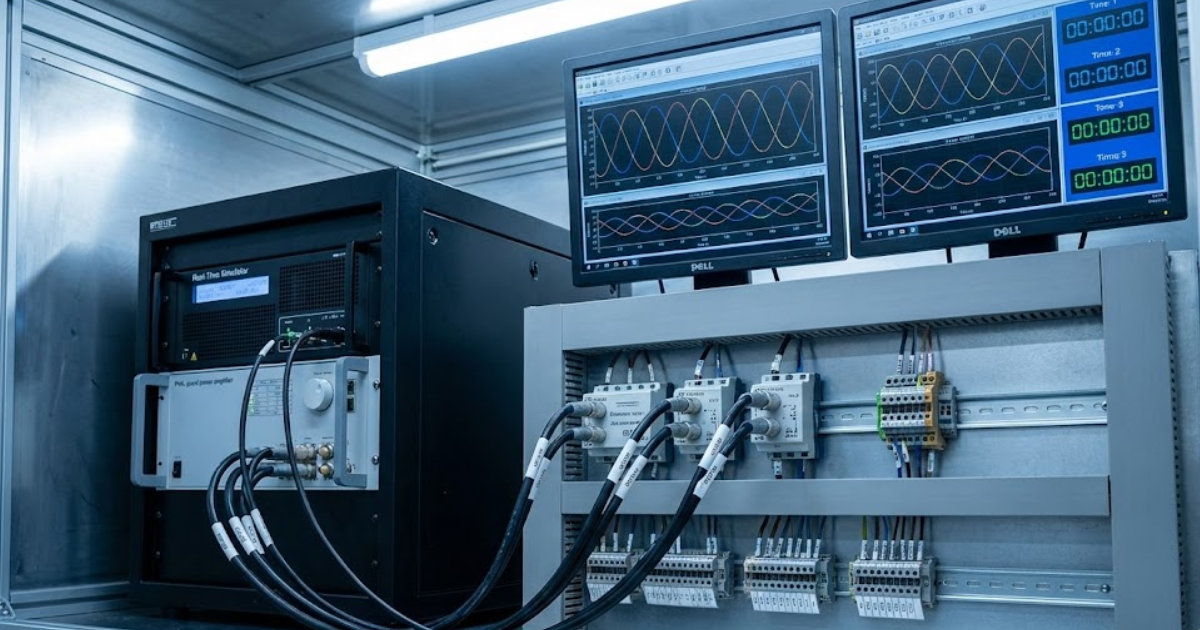
PHIL fidelity is mainly shaped by time step, end-to-end latency, and how the interface algorithm maps simulated quantities to physical signals. The simulator must finish each step before the next deadline, or the loop will jitter and destabilize. The amplifier and sensors must reproduce the bandwidth you care about without saturating. Interface tuning sets the boundary between what is “grid” and what is “hardware.”
Start with a latency budget instead of starting with model detail. Compute time, input and output conversion, amplifier group delay, and sensor filtering add up, and that sum sets the maximum stable loop gain at higher frequencies. A small, stable PHIL simulation with clean measurements will validate more than a huge model that misses deadlines. Fidelity should match the question you’re trying to answer, not the maximum possible model order.
|
Checkpoint |
What you decide early |
What breaks when ignored |
| Time step and solver choice | Pick the smallest step that still runs deterministically | Missed deadlines create jitter that looks like unstable control |
| End-to-end loop latency | Budget compute, conversion, amplifier, and sensor delays | Extra delay erodes phase margin and causes oscillations |
| Amplifier bandwidth and saturation | Match slew rate and harmonic range to your test objectives | Saturation distorts waveforms and hides true protection behavior |
| Sensor range and filtering | Size ranges for faults and choose filters for noise control | Clipping and aliasing create false stability or false trips |
| Interface algorithm selection | Choose voltage type or current type interface for stability | Poor mapping makes the simulator and hardware fight each other |
| Fault and trip coordination | Define what triggers a trip and what state is preserved | Unclear trip logic ruins repeatability and complicates debugging |
Power interface selection for amplifiers, sensors, and protection
Power interface selection sets the physical contract between your simulated grid and the device under test. You choose how the amplifier will be commanded, how voltage and current will be measured, and how fast protection must react. Those choices determine loop stability and the validity of fault behaviour. A good interface makes the hardware “feel” the simulated network without adding hidden dynamics.
Voltage interfaces are intuitive when the simulated grid is stiff, while current interfaces can be more stable when the device controls its own voltage. Sensor placement and isolation must support both normal operation and faults, because transient conditions often contain the most useful validation signals. Protection should be layered, with hardware interlocks that remain effective even if software misbehaves or the model diverges.
Pay special attention to scaling, offsets, and sign conventions. Small errors can look like control instability, and large errors can create unsafe setpoints. Calibration needs to be repeatable and tied to the same measurement chain used during tests, because swapping probes or changing filters changes the loop. A PHIL test bench becomes predictable when interface details are treated as first-class design choices.
Step-by-step workflow to build, tune, and validate PHIL
A reliable PHIL workflow moves from low-energy checks to closed-loop power runs, while you validate timing, scaling, and protection at each step. The first build should target stability and repeatability, not maximum power. Each change should be isolated, measured, and then locked down as a baseline. This approach prevents unstable loops from consuming lab time and confusing results.
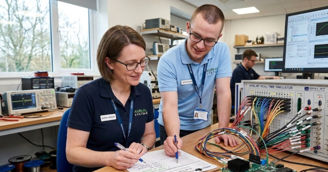
A concrete case helps: a team validating a 50 kW inverter controller can start with a low-voltage power stage, then ramp to full voltage only after timing and protection pass. The workflow begins with open-loop amplifier checks, then sensor calibration, then closed-loop at reduced gain and limited current. Fault cases get added only after stable steady-state operation is repeatable. A real-time simulator from OPAL-RT can run the network model deterministically while you track latency and missed-step counters as acceptance gates.
Validation should include pass criteria that survive scrutiny from both engineering and lab safety roles. Timing measurements need to cover worst-case compute load, not only average load, because the worst case sets stability. Trip behaviour needs to be deterministic, so the same fault produces the same shutdown path each time. When the workflow is disciplined, you’ll trust negative results as much as positive ones, which is the entire point of PHIL simulation.
Common failure modes in PHIL simulation and how to fix
Most PHIL failures come from delay, saturation, or measurement artifacts that the model does not include. Latency pushes phase lag into the loop and can turn a stable plant into an oscillator. Amplifier limits can clip waveforms, which changes harmonics and confuses control behavior. Noise, aliasing, and scaling errors can trigger protections that would never trip in a clean setup.
Stability issues should be handled like a control problem, not a wiring problem. Measure loop delay end to end, then reduce loop gain at frequencies where phase margin collapses, often through interface compensation or filtering. Confirm that the amplifier is operating inside its linear range for the test, because “good enough” headroom at steady state can disappear during a fault. Watch for sensor filter settings that make plots look smooth while hiding unstable content.
Repeatability issues usually trace back to uncontrolled initial conditions and inconsistent trip handling. Define startup sequencing, pre-charge rules, and what states are reset between runs. Log raw sensor values and interface commands alongside simulated states, because debugging needs both sides of the loop. Fixes stick when you treat each failure mode as a test bench requirement that gets verified, not as a one-time patch.
When to choose PHIL instead of CHIL or offline models
“The best PHIL setups feel almost boring during operation, and that boring consistency is what lets you make hard calls with confidence.”
The main difference between PHIL, controller hardware-in-the-loop, and offline simulation is what risk you are retiring. Offline models retire design risk in algorithms and sizing, but they don’t expose the timing and power-path behaviour of hardware. Controller hardware-in-the-loop retires control software and I/O timing risk, but it still keeps power idealized. PHIL retires power-path and protection risk because it forces actual energy exchange.
PHIL is the right choice when your success criteria depend on interactions that only appear under power, like amplifier saturation effects, sensor dynamics, protection coordination, and hardware limits that reshape waveforms. Controller-only testing is usually enough when the power stage is mature and the main uncertainty is software logic and timing. Offline work is usually enough when you’re still exploring architectures and don’t need to validate protection behaviour. Picking PHIL too early wastes effort, while picking it too late pushes power risk into commissioning.
Long-term confidence comes from treating PHIL as an engineering discipline with acceptance gates, not as an occasional lab stunt. Teams that get repeatable PHIL results tend to standardize latency budgets, protection layers, and calibration routines, then reuse them across programs. OPAL-RT fits naturally when you need deterministic real-time execution and a flexible interface to lab power equipment, because repeatability depends on execution details more than on marketing claims.
Real-time solutions across every sector
Explore how OPAL-RT is transforming the world’s most advanced sectors.
Simulation
03 / 11 / 2026
9 Common hardware in the loop testing pitfalls in embedded and control validation
Nine common hardware-in-the-loop testing pitfalls in embedded and control validation, with practical fixes for timing, model fidelity, solver stability, I/O integrity, protocol behaviour, automation repeatability, and configuration traceability.
Power Electronics
03 / 09 / 2026
FPGA vs CPU for real time power electronics simulation
You’ll learn how to choose CPU, FPGA, or a split approach for real-time power electronics HIL simulation using time step targets, latency and jitter needs, switching model fidelity, partitioning, and workflow constraints.

Simulation
03 / 04 / 2026
When to add FPGA acceleration to an existing real time simulator
Engineers can use timing symptoms, workload fit, and migration steps to decide when FPGA acceleration will resolve HIL deadline, latency, and jitter limits in an existing real-time simulator.
EXata CPS has been specifically designed for real-time performance to allow studies of cyberattacks on power systems through the Communication Network layer of any size and connecting to any number of equipment for HIL and PHIL simulations. This is a discrete event simulation toolkit that considers all the inherent physics-based properties that will affect how the network (either wired or wireless) behaves.