Scaling real time simulation from desktop models to full labs
Simulation
02 / 16 / 2026
Key Takeaways
- Successful HIL lab scaling depends on deterministic timing targets, not more channels or bigger racks.
- Partition compute across CPU, FPGA, and networks using a single latency and jitter budget that you can test and enforce.
- Operational controls will determine repeatability, so lock configurations, standardize calibration, and fail tests when timing slips.
Scaling a hardware-in-the-loop lab works when you lock timing, I/O, and model scope before you add racks.
Bugs that slip past early verification get expensive later, and the U.S. economy loses $59.5 billion each year due to inadequate software testing infrastructure. Real-time simulation reduces that risk only when it stays deterministic as complexity rises.
The most scalable approach is disciplined: set hard performance targets first, then partition compute, then engineer the signal path, then decide what model detail belongs in real time. That order feels strict, but it keeps you from “fixing” overruns with ad hoc workarounds that break repeatability. You’ll end up with a lab that runs the same test the same way, every time, across one bench or a full room of racks.
“Teams get stuck during HIL lab scaling when they treat it like a hardware purchase instead of a timing and integration problem.”
Define HIL lab scaling from desktop models to racks
HIL lab scaling means growing from a single desktop model to multiple synchronized real-time targets while keeping closed-loop behaviour stable and repeatable. The success metric is not channel count; it’s deterministic timing, consistent I/O behavior, and test repeatability across stations and operators. Scalable real-time simulation is mostly about managing interfaces and time.
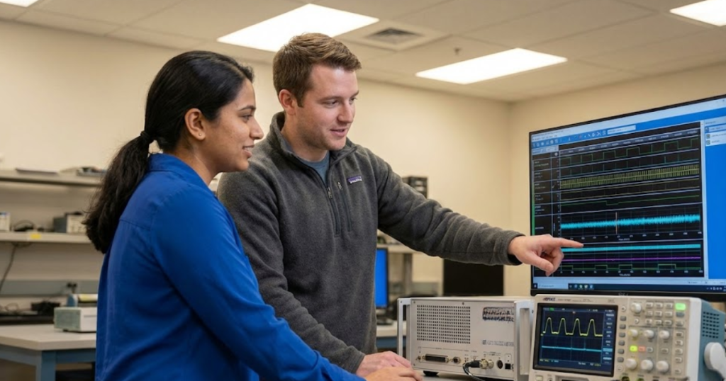
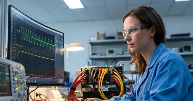
Desktop simulation forgives a lot. Your solver can take a little longer, your OS can schedule another process, and your signals can stay “ideal” because they never hit a wire. A lab does not forgive those choices. The moment you connect hardware, any timing slip shows up as jitter, missed edges, unstable loops, or inconsistent pass fail results across runs.
Scaling also has an organizational meaning: more users, more test assets, more configurations, and more pressure to reuse setups. If your lab can’t reproduce results across two identical benches, adding more racks only multiplies uncertainty. Treat scaling as a system design problem, not an expansion project, and you’ll keep your validation effort credible.
Set real-time performance targets before adding hardware channels
Scaling starts with a performance budget that you can measure and enforce. You need explicit targets for fixed time step, worst-case execution time, I/O latency, jitter limits, and acceptable dropped frames, all tied to the control bandwidth you must validate. Extra channels only help after those limits are clear and verified.
Start by writing down the fastest loop you must close and the timing that loop can tolerate. That statement becomes your lab’s contract: sample time, sensor to compute latency, compute to actuator latency, and allowable jitter. You’ll also need a rule for what happens when timing is violated, because silent overruns create “passing” tests that are not trustworthy.
Once targets exist, scaling becomes a series of checks instead of debates. You can validate a new rack, a new I/O card, or a new model build against the same budget. That is the difference between a lab that grows smoothly and a lab that spends months chasing timing ghosts after every upgrade.
| Scaling checkpoint | What you verify before adding more capacity |
| Fixed step timing | The simulator always finishes each step within the step period. |
| End-to-end latency | Sensor input to actuator output stays within the control loop limit. |
| Jitter tolerance | Timing variation stays below what your controller can handle. |
| I/O fidelity | Signal levels, scaling, and update rates match what hardware expects. |
| Repeatability controls | Test setup, calibration, and configuration produce consistent outcomes. |
| Failure visibility | Overruns and dropped samples are logged and fail tests on purpose. |
Choose simulation partitioning across CPU FPGA and network links
Partitioning is the act of placing each model function where it can meet timing with margin. Fast, simple, and tightly coupled math belongs where determinism is strongest, while slower or less time-critical parts can run on general compute. Network links then become part of the timing budget, not a convenient cable.
A concrete way to think about this is to separate “hard real-time” from “soft real-time.” Switch-level power electronics, encoder edge capture, or very fast protection logic often needs hardware-timed execution. Plant dynamics with longer time constants, supervisory logic, and monitoring can tolerate a looser schedule. A team validating an inverter controller can run the fast switching interface and PWM capture on FPGA while keeping slower thermal limits and fault sequencing on CPU, then validate timing on the same step size used in the rack system.
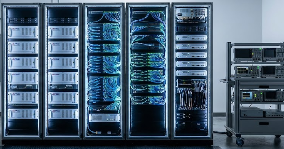
Multi-rack scaling adds one more constraint: clock alignment across targets. Precision time protocol targets submicrosecond synchronization on local networks. That number matters because it frames what “simultaneous” means when two racks must agree on timestamps, event ordering, and fault injection timing.
Plan I/O and signal conditioning for closed-loop tests
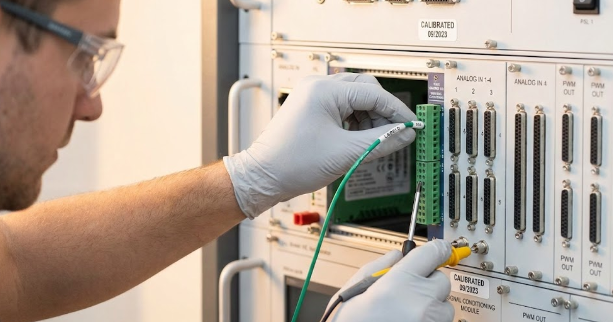
I/O planning is where many desktop models fail in the lab, because wires impose physics. You need a defined signal chain from simulated variable to physical connector, including scaling, filtering, isolation, protection, and calibration. Closed-loop tests only stay trustworthy when the signal path is as engineered as the model.
Start with the DUT interface requirements: voltage and current ranges, input impedance, expected edge rates, grounding scheme, and fault behaviour. Decide what must be measured versus what can be inferred, since measurement adds latency and noise that controllers will react to. Then design signal conditioning so the simulator and the DUT agree on units and timing at every boundary, not just in a spreadsheet.
This is also where toolchain openness matters, since labs rarely stay static. OPAL-RT systems are often deployed with modular I/O and configurable signal paths so teams can adjust channel mix and conditioning without rewriting the entire setup. The practical test is simple: a new channel should be added with the same timing, the same calibration method, and the same logging rules as existing channels.
Scale model fidelity and solver steps without losing determinism
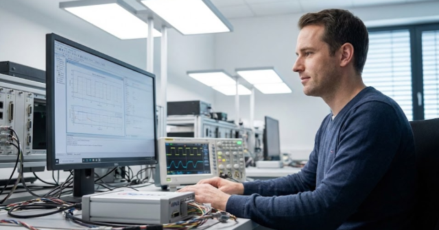
Model fidelity scales safely when you treat compute time as a scarce resource and spend it where it changes test outcomes. Determinism comes first; extra detail only matters if it improves the controller behaviour you are trying to validate. The goal is a model that is “detailed enough” at a step size you can hold, with margin.
Start with the control bandwidth and the signals that drive pass fail decisions. Put fidelity into those paths, then simplify the rest. Replace very stiff dynamics with numerically stable equivalents, avoid algebraic loops that force variable step behaviour, and reduce unnecessary switching detail when an averaged model produces the same control response at your target step.
When you must increase fidelity, treat it like a change request with a timing test attached. Add one improvement, re-measure worst-case execution time, then decide if you need more compute, different partitioning, or a different model form. This keeps “better physics” from silently becoming “unreliable timing,” which is the fastest way to lose confidence in lab results.
“The success metric is not channel count; it’s deterministic timing, consistent I/O behavior, and test repeatability across stations and operators.”
Avoid common HIL lab scaling failures in integration and operations
Most scaling failures are operational, not mathematical. Labs break when timing problems are hidden, configurations drift, calibration becomes tribal knowledge, or test ownership is unclear. You scale a HIL lab by making repeatability a requirement that operations can enforce, not a hope that engineers remember during crunch time.
These are the failure modes that show up first as you move past a single bench:
- Timing overruns get logged but do not fail tests, so bad runs look valid.
- Signal scaling and calibration live in local files, not controlled baselines.
- Network and time sync settings vary across racks, causing subtle offsets.
- Hardware revisions change without a regression plan tied to performance targets.
- Operators run “almost the same” procedures, so results are not comparable.
The fix is boring and effective: treat the lab like production test. Lock configurations, version control test assets, require automated checks for overruns, and standardize calibration. OPAL-RT can fit into that discipline, but the discipline is the real scaling mechanism, and it will outlast any single hardware generation.
Real-time solutions across every sector
Explore how OPAL-RT is transforming the world’s most advanced sectors.
Simulation
02 / 26 / 2026
CPU versus FPGA simulation for high speed motor drive testing
Compares CPU and FPGA real-time simulation for high speed motor drive HIL testing, focusing on timing limits, solver step size, switching fidelity, I/O latency, and acceptance criteria.
Power Electronics
02 / 24 / 2026
Fault tolerant control workflows for multiphase electric drives
Covers how to detect, isolate, and recover from inverter and winding faults in multiphase motor drives, including control reconfiguration, derating limits, and validation with real time models and hardware-in-the-loop tests.
Industry applications
02 / 24 / 2026
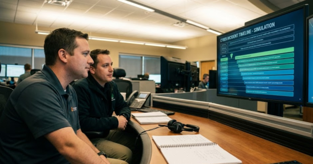
Building Cybersecurity Simulation Training For Utilities
Learn how utilities use cybersecurity simulation training and cyber range simulation to run safe, repeatable OT and IT exercises that improve incident response.
EXata CPS has been specifically designed for real-time performance to allow studies of cyberattacks on power systems through the Communication Network layer of any size and connecting to any number of equipment for HIL and PHIL simulations. This is a discrete event simulation toolkit that considers all the inherent physics-based properties that will affect how the network (either wired or wireless) behaves.