What engineering teams need before launching a motor drive HIL program
Simulation
02 / 10 / 2026

Key Takeaways
- Motor drive HIL readiness starts with clear goals, measurable pass fail metrics, and a controlled scope that matches your highest-risk functions.
- Model fidelity, IO choices, and loop timing must be treated as one closed-loop system, since small latency or scaling errors will create false control problems.
- A repeatable test plan with automation, data capture, and review gates will keep bring up stable and keep teams aligned as control code and hardware change.
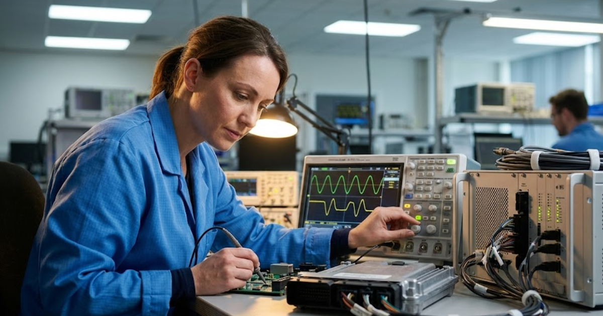
Motor drive HIL programs go smoothly when requirements and timing are locked before any wiring starts.
Motor-driven systems account for about 45% of global electricity consumption, so small control or efficiency mistakes add up quickly. A motor drive hardware in the loop (HIL) setup lets you test controls against a real-time plant model while keeping the power stage safe. That benefit only shows up when the team treats HIL readiness as a systems task, not a lab purchase. You’re building a closed loop with strict timing, strict signals, and strict pass fail criteria.
Teams that succeed decide what “done” means early, then build the model, hardware, timing, and tests to match that definition. Teams that struggle usually skip one of those steps and spend weeks chasing noise, latency, or mismatched assumptions. The difference is discipline, not ambition. If you want HIL to reduce risk instead of adding schedule risk, you need a readiness plan you can execute.
Define motor drive HIL goals, use cases, and success metrics
Your first HIL deliverable is a written target for what you will prove. Define which control functions must run closed loop, what faults you must inject, and what performance boundaries matter. Put numbers on acceptance where you can, but keep them tied to test evidence you can actually capture. Treat “HIL is working” as a set of measurable outcomes.
Start with a short list of questions your team keeps arguing about, then convert each into a testable statement. Typical categories include startup behaviour, torque command tracking, current limits, fault reactions, and safe shutdown. Decide what artifacts count as proof, such as waveforms, logs, or pass fail flags from automated checks. Align those choices with the stage you’re in, since early controller bring up needs different evidence than pre-release validation.
Tradeoffs show up immediately. Narrow goals let you stand up the bench faster, but they can hide failure modes that appear when conditions vary. Broad goals raise modelling and integration effort, and timing issues get harder to isolate. A good compromise is a small set of high-risk functions with clear stop conditions, plus a backlog of “next” items that won’t block initial readiness.
Select target inverter, motor, and load scenarios for HIL
HIL readiness depends on selecting the operating conditions you must cover, not on modelling everything you can imagine. Pick the inverter behaviours, motor type, sensing chain, and load dynamics that most affect control stability and protection logic. Define boundaries for voltage, speed range, and torque direction changes. Then write down which conditions are out of scope for the first phase.
A concrete way to do this is to lock a single baseline scenario and treat it as the reference for every modelling and wiring choice. One practical baseline is a traction inverter feeding a permanent magnet synchronous motor with a resolver interface, plus regenerative braking and field weakening as required behaviours. That single selection forces clarity on which sensors must be emulated, which faults matter, and how you’ll represent load inertia and road load. It also prevents the common failure mode of building a bench that can’t reproduce the behaviour your control team cares about.
Scope control matters more than completeness. If your initial scenario mixes too many sensing options, motor variants, and thermal or saturation effects, you’ll spend time debating model fidelity instead of validating control. If it’s too simple, protection logic and observer tuning look stable on HIL but fail later when conditions shift. Your goal is a scenario set that stresses the controller the same way the hardware will, with the smallest model and wiring set that can do that.
“Motor drive HIL programs go smoothly when requirements and timing are locked before any wiring starts.”
Prepare plant and control models that run in real time
Motor drive HIL only works when both the plant and the controller execute deterministically in real time. That means fixed-step behaviour, bounded computation time, and a clear mapping between model sample times and control loop rates. You also need a plan for what gets simplified and what must stay high fidelity. Model choices should match your goals, not your favourite tool.
Plant modelling should prioritize electrical dynamics that shape current control, plus mechanical dynamics that shape speed and torque response. Switching-level detail can be useful, but average-value representations often get you to stable closed-loop testing sooner, especially during early bring up. Whatever level you choose, validate steady-state behaviour and transients against a known reference before closing the loop. Controller modelling must include the same numerical limits, discretization, and saturation behaviour that will exist on the target processor.
The implication is simple: if the model can’t meet the time budget, the loop will lie to you. When execution overruns, you’ll see false oscillations, delayed protection triggers, and confusing sensitivity to solver settings. Set a performance budget early and treat it like a hard requirement. You’ll save more time cutting model complexity in the right place than you will fighting timing debt later.
Specify HIL hardware, IO, and signal conditioning requirements
Hardware readiness is about accurate signals, safe power interfaces, and enough headroom for timing and expansion. Define every input and output, the signal type, the update rate, and the expected fault behaviour. Plan isolation and grounding up front, since motor drive benches punish sloppy wiring. Your HIL hardware choice should follow these constraints, not lead them.
You’ll also need a clear boundary between what the HIL simulates and what external hardware provides, especially for sensors and gate commands. When teams use platforms such as OPAL-RT, the most useful early step is mapping every channel to an electrical standard and a calibration check, then confirming the required latencies are achievable with the chosen IO modules. Signal conditioning is not an accessory; it is part of the plant interface. If the controller “sees” the wrong scaling or filtering, you won’t know if failures are control bugs or bench artifacts.
- Document each channel with units, scaling, and expected ranges
- Choose isolation and protection for every high-energy interface
- Define sensor emulation needs for position, current, and voltage
- Confirm digital outputs match gate driver input requirements
- Plan calibration checks you can repeat after every wiring change
Verify timing, latency, and synchronization across the full loop
Timing is the hidden contract that makes motor drive HIL credible. Verify the end-to-end loop from controller output, through I/O, through the plant model, and back to controller inputs. Measure latency and jitter, then confirm they stay within what your control design assumes. Synchronization across analog, digital, and encoder style signals must also be consistent.
Start with a timing budget that allocates margin to each segment, then test each segment independently before you close the loop. Use step responses and timestamped logging so you can see delay clearly, not just infer it from waveform shape. Confirm that sampling, PWM update, and sensor feedback timing line up with the controller’s scheduling assumptions. If your controller expects coherent sampling but your bench returns skewed signals, tuning will look unstable even when the control code is fine.
| Readiness area | What “ready” looks like | What fails when it is missing |
| Loop timing budget | The loop has measured margin against worst-case execution time. | Overruns show up as false instability and misleading protection trips. |
| Signal integrity | Scaling, filtering, and noise levels match what the controller expects. | Tuning becomes guesswork because the bench adds artifacts. |
| Synchronization | Feedback signals align consistently across sample domains. | Observers and estimators drift due to timing skew, not plant physics. |
| Fault insertion control | Faults are repeatable with timestamps and clear reset behaviour. | Safety logic cannot be validated because triggers are inconsistent. |
| Data capture plan | Logs capture enough context to explain every fail. | Teams rerun tests repeatedly because root cause cannot be proven. |
| Configuration control | Model, firmware, and wiring revisions are tracked as a single baseline. | Results cannot be compared across days, so progress stalls. |
Build a test plan with automation, data capture, and review gates
A motor drive HIL program starts delivering value when tests run the same way every time and produce evidence people trust. Define test cases from your goals, then add automation hooks so runs are repeatable and reviewable. Set review gates that stop the bench from becoming a demo rig with no accountability. Treat the test plan as a product that needs upkeep.
Automation matters because manual testing hides regression, and regression is what burns schedules. Software defects already create a measurable economic burden, with an estimated $59.5 billion annual cost in the United States tied to software errors and inadequate testing practices. A HIL bench without automated checks often becomes a high-effort way to repeat the same bring up steps. A HIL bench with automation becomes a safety net that catches changes in control gains, scaling, and timing.
Review gates keep everyone honest. Define what must pass before you expand scope, such as timing margin, stable current control, and repeatable fault reactions. Store logs in a place where both control and test teams can access them, and agree on naming and version rules. If you can’t reproduce a failure within a day, the plan needs better triggers, better capture, or tighter configuration control.
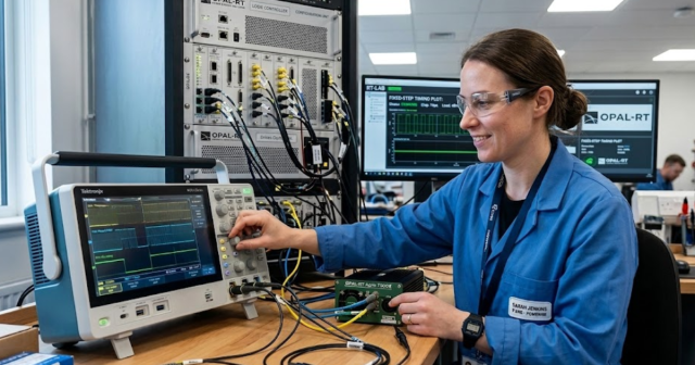
“Timing is the hidden contract that makes motor drive HIL credible.”
Prevent common motor drive HIL implementation failures during bring up
Bring up failures usually trace back to mismatched assumptions, not exotic physics. Teams wire signals that don’t match units, close loops before timing is stable, or chase noise that is really a grounding issue. Prevention comes from staged integration, clear baselines, and fast checks that prove each layer works. When you slow down at the right moments, the bench speeds up overall.
Start with open-loop checks that validate every signal path, then move to closed-loop control with conservative limits and clear abort conditions. Keep a single “golden” configuration that everyone treats as the reference, even if experiments happen on the side. When a failure appears, isolate it with one change at a time, and require evidence that the change fixed the root cause rather than masking symptoms. Timing and scaling problems will imitate control design issues so well that you’ll waste days unless your process forces separation.
Long-term success comes from treating readiness as a shared responsibility across controls, power electronics, and test. OPAL-RT teams often see the best outcomes when the bench is managed like a system, with measured timing, controlled wiring, and test gates that keep scope honest. If you do that work up front, HIL turns into a repeatable validation asset instead of a recurring integration fire drill. That discipline is what earns confidence when schedules get tight and changes keep coming.
Real-time solutions across every sector
Explore how OPAL-RT is transforming the world’s most advanced sectors.
Industry applications, Simulation
03 / 31 / 2026
Managing high-frequency switching in real-time EMT simulation
Precision in testing complex power systems is essential to avoid failures, accelerate innovation, and integrate new technologies safely.

Simulation
03 / 30 / 2026
Understanding timestep requirements for modern power converters
Practical criteria for selecting EMT and real time simulation timesteps for power converters, covering switching resolution, control and PWM timing alignment, multirate approaches, and verification checks.

Energy, Industry applications, Simulation
03 / 29 / 2026
Validating data center energy management systems using real-time HIL
This piece explains how AI workload variability affects data centre power stability and how closed-loop HIL testing helps validate EMS control behaviour under site and grid stress.
EXata CPS has been specifically designed for real-time performance to allow studies of cyberattacks on power systems through the Communication Network layer of any size and connecting to any number of equipment for HIL and PHIL simulations. This is a discrete event simulation toolkit that considers all the inherent physics-based properties that will affect how the network (either wired or wireless) behaves.