A complete guide to real time power electronics simulation for control engineers
Power Electronics, Simulation
01 / 20 / 2026

Key Takeaways
- Real time simulation earns trust when timing, latency, and compute budgets are treated as design inputs.
- Model fidelity should follow the test objective, with timing nonidealities and sensor behaviour captured before extra physics detail.
- Staged testing from simplified plants to closed-loop controller runs will surface faults earlier than late hardware integration.
Real time power electronics simulation shows you if a controller will stay stable once clock time and I/O delays show up. You get a plant model that runs on schedule, step after step, with no “extra time” allowed. That forces the same sampling, computation, and protection timing you will face on hardware. Faster confidence comes from seeing timing faults early, not from polishing plots.
Late fault discovery is expensive across engineering work, and software is a clear warning sign. Flaws in software still cost the U.S. economy about $59.5 billion each year. Control firmware hits the same trap when missed deadlines, quantization, or limiter logic stay hidden until bring-up. Real time simulation pulls those issues forward so you can fix them while design choices are still cheap.
Real time power electronics simulation answers control design timing limits
Real time power electronics simulation executes a converter model at the same pace as wall clock time. Each fixed step must finish before the next step starts, so timing becomes a hard requirement. You can close the loop with control code and I/O that behave like a bench setup. The output is a measurable picture of stability with realistic delay.
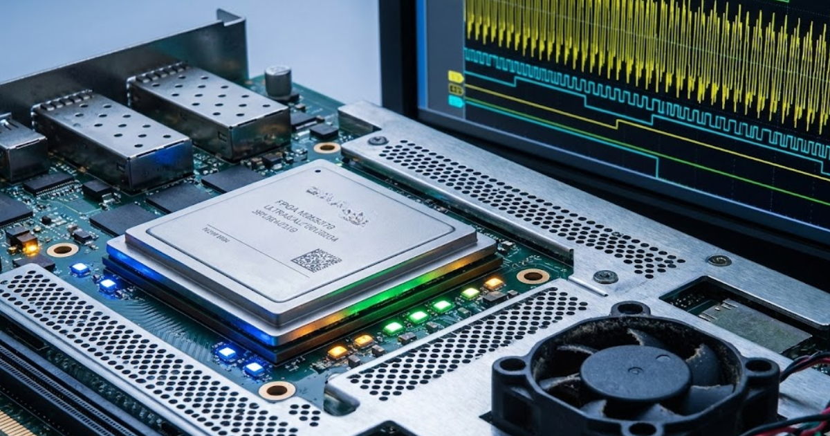
Picture a 100 kHz buck converter with a 20 kHz digital voltage loop. Offline runs often assume instant switching events and perfect measurements, so the controller sees clean signals. A real time run forces PWM updates, ADC sampling, and computation to land on exact ticks. A harmless looking transient peak will turn into duty clamping, current limiting, or a discrete oscillation.
Timing constraints change how you design from day one. You will budget compute time, align sample rates, and account for I/O latency in the loop gain. Real time simulation makes those budgets visible instead of implied. That clarity helps you pick what must run fast and what can run slower without breaking control behaviour.
“Timing constraints change how you design from day one.”
Offline simulation gaps that appear once switching meets control loops
Offline simulation is great for physics detail, but it rarely punishes bad schedules. Variable step solvers take tiny steps around switching and large steps elsewhere, so timing pressure disappears. Ideal switches and perfect sensors slip in and make control look cleaner than it is. The first hardware run then becomes the timing audit you skipped.
Take a motor inverter current loop tuned on an averaged bridge model. The current tracks nicely, and the bandwidth looks generous on a frequency plot. A switched model with discrete sampling shows ripple folding into the sampled current and corrupting the error signal. One sample of delay can turn a quiet loop into subharmonics and torque ripple.
Offline and real time runs answer different questions, and that difference is useful. Offline runs work best for long transients, thermal limits, and wide parameter sweeps. Real time runs work best for scheduling, quantization, delays, and protection timing. You will move faster when you plan both from the start.

Fidelity requirements that separate useful real time models from noise
Fidelity in real time simulation is a budget tied to one test. Keep detail that changes the controller outcome and drop the rest. Timing errors and sensor behaviour matter before loss curves. A model earns trust when it answers one question reliably.
A grid tied inverter shows the trade. Outer loop tuning can use an averaged stage because ripple is not the driver. Inner current loop checks need a switched bridge and the same sample clock as the controller. Protection checks need sensor delay and clamps more than fine device physics.
| What you set first | What you verify next |
| Step matches clocks. | CPU margin stays. |
| Switching targets ripple. | Ripple matches probes. |
| Averaging targets slow loops. | Margins hold with delay. |
| Dead time is modelled. | Duty avoids saturation. |
| Sensors include filtering. | Estimates stay stable. |
Fidelity work ends when results repeat. Extra detail after that adds noise and slows execution. Too little detail hides the fault you came to test. The best model is the one you can explain.
Numerical methods that hold stability at microsecond time steps
Microsecond steps reveal numerical weakness fast. Real time simulation uses fixed step integration, so solver choice sets stability. Stiff networks from tiny inductances, parasitic capacitances, and ideal switches will dominate the step. Stable results come from choosing a method that matches the circuit.
A half bridge feeding an LC filter shows the trap. An explicit update can inject energy and grow an oscillation that looks like a control fault. A trapezoidal or backward Euler update damps that numerical energy at the same step. Small, justified damping in the circuit can tame stiffness without masking control behaviour.
A few checks prevent solver trouble from masquerading as controller trouble:
- Pick a step size that resolves switching edges.
- Break algebraic loops so order is clear.
- Add small damping where ideal parts stiffen.
- Align control updates to integer steps.
- Track numerical energy drift.
Good numerics saves time because phantom instability disappears. You stop tuning against a solver artefact. Step and method changes should not flip a stable design into chaos. That repeatability is what makes results worth trusting.
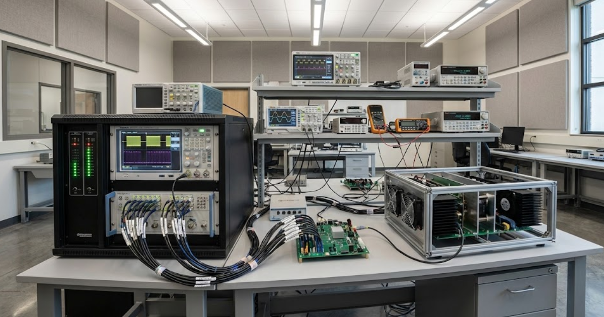
Hardware and I/O constraints that shape practical real time setups
I/O turns a simulator into a closed loop test bench, and it adds delay. Analogue channels have sample and hold behaviour, digital lines have edge capture limits, and every path has latency. Those delays sit inside your loop and shift phase like a filter. Trust grows when you measure I/O timing and model it.
A practical case is a controller that reads phase currents and writes PWM gate commands. The input path includes anti alias filtering and conversion delay, and the output path includes isolation delay and edge timing limits. A protection feature that trips in 2 microseconds will fail if the I/O updates every 10 microseconds. Fixing that means adjusting the schedule, the hardware interface, or the protection goal.
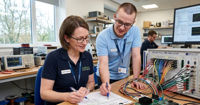
Execution detail matters more than branding, but platform behaviour still shapes your tests. OPAL-RT systems are often configured with deterministic I/O scheduling so controller sampling and plant updates stay aligned. The same discipline applies on any rig you build. Write down end to end latency so results stay comparable.
Where real time simulation fits across design verification and test stages
Real time simulation works as a progression that tightens realism as risk rises. Early checks focus on control logic, limits, and margins, so simplified plants are enough. Mid checks add switching, sampling, and I/O delays to expose ripple and timing faults. Late checks close the loop with controller hardware or compiled code and push faults through protection.
A power factor correction design illustrates a sensible sequence. The voltage loop can be tuned with an averaged boost model to get stable energy balance and clean transients. Switching detail then checks current ripple, sensor filtering, and PWM timing limits. Hardware in the loop tests follow, where the controller runs its real scheduler and trips its real protection logic.
Reliability stakes justify this staged effort outside the lab. Power outages cost U.S. businesses as much as $150 billion per year. Control and protection mistakes will feed the same outage pattern through trips, restarts, and poor recovery logic. Real time simulation is where you rehearse those edge cases before a site forces the lesson.
“Confidence breaks when simulation becomes reassurance instead of a test.”
Common misuse patterns that reduce confidence in simulation results
Confidence breaks when simulation becomes reassurance instead of a test. Ignoring delay, quantization, and limiter behaviour will flatter the controller and punish you later. Skipping fault cases makes protection look perfect until the first abnormal condition. A trustworthy workflow treats every assumption as a measured parameter.
One common misuse is tuning on an averaged plant and treating the gains as final. Switching ripple, dead time, and ADC delay change phase and effective gain, so the tuned bandwidth will not hold. Another misuse is running a “real time” case with a step so large that PWM becomes a slow duty signal. Quantization, saturation, and missed deadlines also get ignored when the control code is replaced with ideal blocks.
A clean test habit feels strict, and it pays off. You will treat timing, I/O, and numerics as design inputs and keep a short record of delays and limits used in each run. OPAL-RT can support that discipline by making deterministic execution and latency visible, but the outcome comes from your choices. Engineers who measure, document, and repeat core fault cases will earn confidence that survives hardware.
Real-time solutions across every sector
Explore how OPAL-RT is transforming the world’s most advanced sectors.
Simulation
03 / 11 / 2026
9 Common hardware in the loop testing pitfalls in embedded and control validation
Nine common hardware-in-the-loop testing pitfalls in embedded and control validation, with practical fixes for timing, model fidelity, solver stability, I/O integrity, protocol behaviour, automation repeatability, and configuration traceability.

Power Electronics
03 / 09 / 2026
FPGA vs CPU for real time power electronics simulation
You’ll learn how to choose CPU, FPGA, or a split approach for real-time power electronics HIL simulation using time step targets, latency and jitter needs, switching model fidelity, partitioning, and workflow constraints.

Simulation
03 / 04 / 2026
When to add FPGA acceleration to an existing real time simulator
Engineers can use timing symptoms, workload fit, and migration steps to decide when FPGA acceleration will resolve HIL deadline, latency, and jitter limits in an existing real-time simulator.
EXata CPS has been specifically designed for real-time performance to allow studies of cyberattacks on power systems through the Communication Network layer of any size and connecting to any number of equipment for HIL and PHIL simulations. This is a discrete event simulation toolkit that considers all the inherent physics-based properties that will affect how the network (either wired or wireless) behaves.