Why high frequency SiC and GaN converters outrun real-time simulation
Power Electronics
11 / 01 / 2026

Key Takeaways
- SiC and GaN converters switching between 200 kHz and 1 MHz push their dynamics past what classic real-time solvers were built to resolve.
- Sub-50 ns timesteps and five to ten times oversampling are now the baseline for faithful high frequency converter models.
- Solvers that need hand tuning or cap switch count push engineers to test a simplified converter instead of the one they’ll build.
SiC and GaN converters now switch faster than most real-time solvers were designed to follow, and engineers who keep validating them on those solvers end up testing a simplified converter instead of the one they intend to build.
The stakes are rising with the volume of power flowing through these devices. Roughly 70% of all electrical energy already passes through power electronics at some point between generation and use, and wide bandgap semiconductors are taking a growing share of those conversion stages in chargers, storage, data centres and aircraft.
Real-time simulation has kept up with every previous generation of power electronics. The jump to converters switching between 200 kHz and 1 MHz is different, because it breaks the assumptions about timestep, tuning and topology size that classic solvers were built on.
Why SiC and GaN push switching frequency past classic solvers
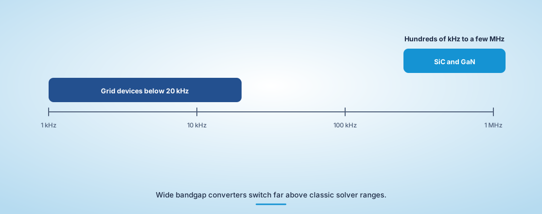
SiC and GaN devices switch with far lower losses than silicon, so designers raise switching frequency to shrink magnetics, capacitors and enclosures. That moves the converter’s important dynamics into a time scale where classic real-time solvers, built for silicon designs switching at tens of kilohertz, can’t resolve them faithfully.
The gap is wide. Most three-phase grid-connected devices operate below 20 kHz, while wide bandgap circuits run at hundreds of kilohertz to a few megahertz. A solver that comfortably covered the first group is working an order of magnitude outside its design range on the second.
Resonant and bidirectional topologies make the problem sharper. LLC, CLLC and dual active bridge converters rely on precise timing between switching edges and resonant currents, and small timing errors in the model change the soft-switching behaviour the controller depends on.
What timestep a 1 MHz converter actually needs
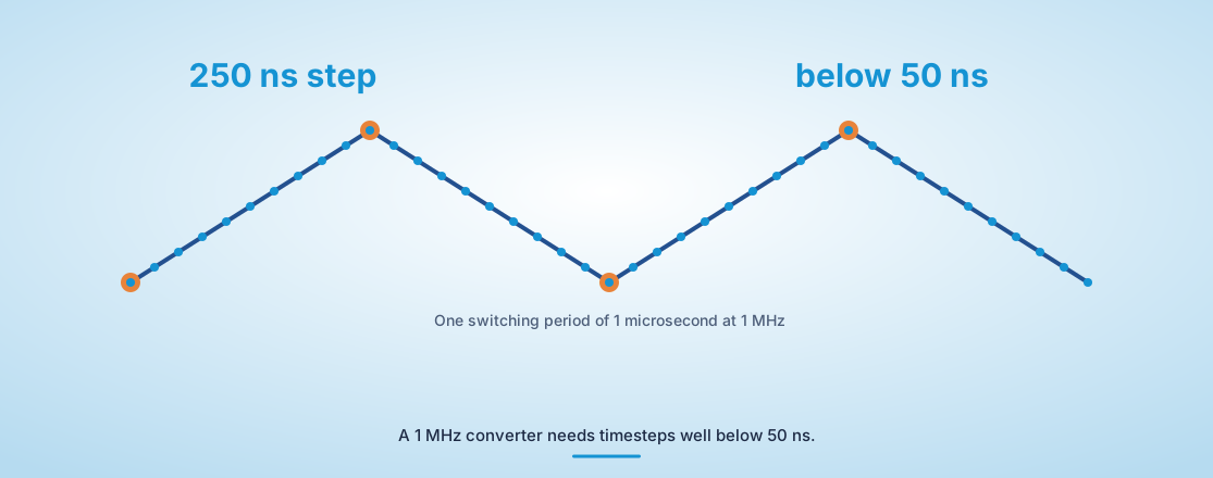
A converter switching at 1 MHz has a switching period of 1 microsecond, so a real-time model needs a timestep well below 50 nanoseconds to place switching events, dead time and resonant transitions accurately. A 250 nanosecond timestep, common on older FPGA solvers, sees only four samples per period.
Four samples can’t represent a resonant current, a dead time of a few tens of nanoseconds or the zero voltage switching window a controller is trying to hit. The model still produces a waveform, but it describes a converter that doesn’t exist, and the controller tuned against it will behave differently on the bench.
How oversampling recovers detail a fixed timestep misses
Oversampling recovers detail by sampling the controller’s gate signals many times within each solver timestep, so switching events are placed at their true instant instead of being rounded to the next step. Engineers now look for five to ten times oversampling on high frequency converter models.
The effect is most visible in dead time. Without oversampling, a gate edge that arrives 12 nanoseconds into a 50 nanosecond step is treated as if it arrived at the end of the step, which shifts current and distorts the voltage the controller measures.
Oversampling also matters for the controller’s view of the plant. Digital controllers sample currents and voltages at specific instants, often synchronized to the PWM carrier, and if the model’s events are rounded, those samples land on the wrong part of the waveform.
Combined with a short timestep, oversampling is what lets a real-time model reproduce the converter the designer drew instead of a smoothed approximation of it.
“Weeks disappear into solver work that doesn’t improve the product.”
Why hand tuning a solver becomes the hidden schedule cost
Hand tuning becomes a hidden schedule cost because many real-time converter solvers need engineers to adjust switch models, damping and discretization for each topology and operating point. Every change to the circuit can restart that work, and the tuning itself can mask real behaviour.
Consider a team validating a CLLC converter for a bidirectional charger. Each time the resonant tank values change during design, the solver parameters have to be revisited to keep the model stable across forward and reverse power flow. Weeks disappear into solver work that doesn’t improve the product.
“The model still produces a waveform, but it describes a converter that doesn’t exist, and the controller tuned against it will behave differently on the bench.”
Where topology limits force engineers to simplify the design
Topology limits force simplification when a solver can only handle a fixed number of switches or a narrow set of circuit structures. Engineers then reduce the converter to fit the tool, merging stages or idealizing parts, and test a design that differs from the one they’ll build.
Modern wide bandgap designs often need 10 to 13 switches in a single topology, especially in matrix converters, multi-port storage interfaces and bidirectional chargers. Simplifications that drop switches or merge phases tend to hide exactly the interactions the controller has to manage.
The designs most often cut down to fit a solver share a few traits, and each one hides a different control risk when it’s simplified.
- Matrix converters that switch every input phase to every output phase
- Multi-port interfaces linking a battery, a solar string and the grid
- Bidirectional CLLC chargers with resonant tanks on both sides
- Interleaved stages that cancel ripple through precise phase shifts
- Multilevel inverters with flying capacitors that need active balancing
The cost appears late. A controller that passed HIL on a simplified model meets the full circuit on the bench and shows instabilities nobody predicted, which pushes validation back into the expensive hardware phase it was meant to replace.
What engineers now need from a real-time converter solver
Engineers now need a real-time converter solver that runs timesteps below 50 nanoseconds, oversamples gate signals by five to ten times, accepts topologies with a dozen or more switches without hand tuning and behaves consistently across the whole operating envelope. Anything less pushes validation back onto hardware.
Those requirements read like a buying checklist, and teams evaluating platforms are using them that way. Engineers working with OPAL-RT have started framing solver evaluations around the converter they intend to build, then checking that the model holds its behaviour from light load to full power in both directions.
The table summarizes the requirements and why each matters.
| Requirement | Why it matters for SiC and GaN converters |
| Timestep below 50 ns | Resonant currents and switching transitions are resolved at megahertz frequencies |
| Five to ten times oversampling | Gate edges and dead time land at their true instants instead of the next step |
| Topologies with 10 to 13 switches | The full converter is tested instead of a simplified substitute |
| No per-topology hand tuning | Design changes don’t restart weeks of solver adjustment |
| Consistent behaviour across the envelope | Light load, full power and reverse flow are all trustworthy test points |
Validating the converter you intend to build
Validating the converter you intend to build means the real-time model matches the real circuit, at its real switching frequency, across its real operating range. That’s the only basis on which HIL results can replace bench time, and it’s the standard high frequency power electronics now has to meet.
We’ve seen the gap between simplified models and real circuits cost converter programs months of late debugging. OPAL-RT built the High Speed Converter Solver around this problem, with a 32 nanosecond timestep and 4 nanosecond internal oversampling, so LLC, dual active bridge, matrix and CLLC designs run as drawn. The full story is in Power in Mind Volume 12, alongside the issue’s other features on electrification testing.

Power Systems
11 / 13 / 2026
Grid forming inverters, how they work and how to test them
A technical explainer on how grid forming inverters and their control loops work, and how to test grid forming control through faults, islanding and weak grids.

Automotive
11 / 08 / 2026
Active vs passive cell balancing and how to validate balancing logic before pack build
A comparison of active and passive cell balancing in battery packs and a practical guide to validating balancing logic on HIL before pack build.

Power Systems
11 / 03 / 2026
Medium voltage and grid interactive UPS systems for data centers
An engineering guide to medium voltage and grid interactive UPS systems for data centres, covering static transfer switches, modular designs and pre-commissioning validation.