
Key Takeaways
- Use cloud simulation to scale test coverage and cut wait time only when each run has clear acceptance checks.
- Keep cloud results trustworthy with reproducible execution using pinned solver settings, controlled versions, and automated pass fail outputs.
- Plan upfront for spend limits, licensing, and security, then shift timing-critical validation to deterministic real-time testing.
It works best when you treat it as elastic compute for repeated, measurable checks, not as a replacement for disciplined modelling or lab testing. Public cloud end-user spending is projected to reach $679 billion in 2024, which signals that elastic compute has become a standard part of engineering operations, not a niche tool. The practical takeaway is simple: cloud simulation pays off when you use scale to increase test coverage and shorten wait time between design decisions.
You’ll get the most value when cloud runs are tied to clear acceptance criteria, version control, and repeatable execution. That stance also keeps expectations grounded because power electronics simulation is sensitive to solver settings, switching detail, and control timing. When those choices are managed well, cloud-based power electronics workflows can move from “we ran a model” to “we can trust the trend across corners.”
“Cloud simulation gives you faster validation loops for power electronics designs.”
What is cloud simulation for power electronics workflows
Cloud simulation for power electronics means running your converter, motor drive, or grid interface models on remote compute instead of a local workstation. You send the model, inputs, and run script to a managed cluster or virtual machines. Results come back as waveforms, logs, and pass fail flags. The purpose is repeatable execution at scale, not just remote access.
Most teams use it for two distinct modes. Batch mode runs many independent jobs, such as parameter sweeps or regression sets, and returns results after completion. Interactive mode supports shorter runs with tighter human feedback, often through a remote desktop or notebook workflow. A smaller slice of use cases targets real-time behaviour, but that demands tight control of step size, timing, and I/O pathways.
The key shift is that compute becomes a variable you can allocate per question. If a single high-fidelity switching model takes hours, you can run more cases in parallel rather than waiting for serial runs on one machine. You still own correctness, though, so cloud usage needs clear model ownership and a defined “done” condition for each run.
When cloud platforms cut simulation time and iteration cycles
Cloud platforms cut simulation time when your bottleneck is total compute throughput, not human debugging. Parallel runs turn a long queue of cases into a short wall-clock batch. Elastic sizing also helps when model size spikes due to finer time steps, more switching detail, or longer transients. The win is fewer calendar days lost to waiting.
Speedups are most reliable for workloads that scale out cleanly. Independent jobs, such as Monte Carlo sampling, corner sweeps, and controller gain searches, map well to many cores and nodes. Longer transient studies also benefit when you can allocate more memory and avoid local resource contention. Interactive tuning improves too, but only if you keep the feedback loop tight and the run setup consistent.
|
Simulation goal |
Cloud approach that tends to fit |
What to watch before scaling up |
| High coverage across operating corners | Many parallel batch jobs with strict version pinning | Consistent pass fail checks so results stay comparable |
| Long transients with fine time steps | Larger instances with more memory per run | Cost growth can outpace the time saved if runs are open-ended |
| Controller tuning against a stable plant model | Automated parameter search with bounded ranges | Unbounded search spaces produce noise, not learning |
| Regression testing after each model change | Scheduled runs triggered by version control events | Licensing and concurrency limits can become the new bottleneck |
| Team collaboration across sites | Shared run artifacts and standardized run scripts | Access control must match IP sensitivity and data residency rules |
“You’re selecting an execution system, not just servers.”
Cloud speed is also a planning problem. If you run without caps, compute growth will look like “more speed” right up until the invoice arrives. Teams that get consistent cycle-time gains set job timeouts, define a minimal result set, and decide upfront which questions need switching detail versus averaged models.
Model setup changes needed for accurate cloud execution
Accurate cloud execution depends on reproducibility, not location. Your model must run the same way every time, with dependencies, solver settings, and inputs fully specified. You also need clean separation between model code and run configuration so automation can work. When you remove hidden state, cloud runs stop producing “mystery differences.”
- Pin solver type, step size, and tolerances so results remain comparable
- Lock model and library versions and record them with each run artifact
- Automate run setup and teardown so humans do not hand-edit parameters
- Capture waveforms, events, and metadata needed to debug a failed case
- Define acceptance checks that turn raw traces into pass fail outcomes
Power electronics models amplify small setup differences because switching edges and control timing can shift with small numerical changes. If your model uses variable-step methods locally, you’ll need a deliberate decision about when variable step is acceptable and when it will hide timing issues. Floating-point behaviour can also differ across instance types, which matters if your control logic depends on tight thresholds.
A practical guardrail is to keep two model tiers. One tier is a fast screening model used for coverage and early sensitivity checks. The other tier is a high-fidelity model used for final verification of waveform limits, protection behavior, and control stability. Cloud compute helps only when both tiers are defined and you know which tier answers each question.
Using cloud runs to validate controls and protection logic

Cloud runs help validate control and protection logic by exercising the same controller across a broad set of operating points and fault conditions. You run closed-loop tests, collect objective checks, and flag edge cases early. That builds confidence before you spend lab time wiring hardware and chasing issues that were visible in simulation. The result is tighter, calmer lab sessions.
A concrete workflow is a three-phase silicon carbide traction inverter control being validated across voltage and load corners. You can execute hundreds of runs that vary DC bus voltage, motor speed, and temperature-dependent device parameters, then inject events such as phase current sensor bias and short-duration overcurrent. The goal is to confirm that current limiting triggers at the intended threshold, that the shutdown sequence is stable, and that restart logic does not chatter. When the run set is defined well, every control change produces a clear delta in pass fail outcomes.
Cloud validation works best when you treat it like test engineering, not like plotting. You’ll want a small set of numeric checks, such as overshoot limits, settling time bounds, and protection response time windows, so you can compare runs without eyeballing every trace. You’ll also want traceability so a failed case can be reproduced exactly, including the model revision and input seed.
After the cloud run set is stable, the next step is closing the loop with hardware timing. Teams often move the same controller into a real-time simulator for hardware-in-the-loop testing, where I/O and execution timing are constrained and measurable. OPAL-RT systems are commonly used at that stage because they focus on deterministic real-time execution while still working with standard modeling toolchains. Cloud simulation and HIL are strongest as a staged flow, with each stage answering a different kind of risk.
Limits, costs, and security constraints you must plan for

Cloud simulation has limits that show up as cost volatility, latency, licensing friction, and security requirements. Costs rise fast when runs are long, high-fidelity, and unconstrained. Latency makes cloud a poor fit for direct interaction with physical lab hardware in tight loops. Security planning matters because model files and test vectors often contain core IP.
Compute also has a physical footprint, which affects governance and budgeting. Data centers used about 460 TWh of electricity in 2022, a reminder that “run everything” has a real cost and should be reserved for questions that change engineering choices. Treat that as a forcing function for prioritization. If a run does not change a design decision, it should not be scaled out.
Security and compliance come down to basic controls executed consistently. You’ll want identity and access management tied to roles, encryption for data at rest and in transit, and clear data retention rules for artifacts. Data residency also matters for regulated projects, so you need a documented answer for where simulations run and where results are stored. Cost controls should be just as strict, with quotas, tagging, and alerts so the team sees spend in near real time.
Choosing a cloud simulation stack for power electronics teams
Choosing a cloud simulation stack comes down to fit between workload type, model fidelity, and validation governance. You need a path for batch scale, a path for repeatable regression, and a path that connects to lab validation when timing and I/O become the focus. Integration matters more than raw compute because simulations only count when results are trusted. You’re selecting an execution system, not just servers.
Start with three decisions you can defend. Decide which models will be run in batch at scale and which require hands-on interaction. Decide how results become pass fail outcomes, since plots do not scale to hundreds of cases. Decide how model revisions, solver settings, and run scripts are controlled so runs remain comparable over time, even as the team changes.
Keep the final judgment grounded in execution discipline. Cloud simulation will pay off when you standardize run inputs, bound compute, and promote only the tests that reduce lab risk. When you pair that with deterministic validation on real-time platforms, you get a workflow that respects both scale and timing. OPAL-RT fits naturally for teams that want that second stage without locking themselves into a narrow toolchain, as long as the same rigor is applied to models, test criteria, and change control.
Real-time solutions across every sector
Explore how OPAL-RT is transforming the world’s most advanced sectors.

Simulation
02 / 26 / 2026
CPU versus FPGA simulation for high speed motor drive testing
Compares CPU and FPGA real-time simulation for high speed motor drive HIL testing, focusing on timing limits, solver step size, switching fidelity, I/O latency, and acceptance criteria.

Power Electronics
02 / 24 / 2026
Fault tolerant control workflows for multiphase electric drives
Covers how to detect, isolate, and recover from inverter and winding faults in multiphase motor drives, including control reconfiguration, derating limits, and validation with real time models and hardware-in-the-loop tests.
Industry applications
02 / 24 / 2026
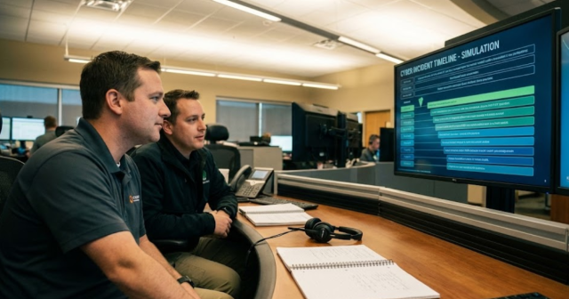
Building Cybersecurity Simulation Training For Utilities
Learn how utilities use cybersecurity simulation training and cyber range simulation to run safe, repeatable OT and IT exercises that improve incident response.
EXata CPS has been specifically designed for real-time performance to allow studies of cyberattacks on power systems through the Communication Network layer of any size and connecting to any number of equipment for HIL and PHIL simulations. This is a discrete event simulation toolkit that considers all the inherent physics-based properties that will affect how the network (either wired or wireless) behaves.