Key Takeaways
- Use SIL to stabilize control logic and interfaces, then use HIL to prove timing, I/O correctness, and safe failure handling under deterministic execution.
- Lock fidelity, step size, and risk targets early, since electrified systems punish late changes in model detail, hardware I/O scope, and safety interlocks.
- Build confidence through automation and repeatability, with versioned models, controlled fault injection, and consistent result reviews that reveal regressions fast.
You can reach release-ready confidence in electrified controls only when SIL and HIL tests stay disciplined and repeatable.
Electric car sales reached nearly 14 million in 2023, and that volume raises the cost of getting control logic wrong. Electrified systems mix fast-switching power electronics with safety logic, sensor conditioning, and network traffic, all under tight timing. That mix makes late integration surprises common when teams treat testing as a single milestone. A staged plan that starts with software-in-the-loop and earns its way to hardware-in-the-loop prevents most of that churn.
The practical stance is simple: treat real-time control testing as a chain of proof, not a single tool choice.
Software-in-the-loop proves algorithms and interfaces cheaply, then hardware-in-the-loop proves timing, I/O, and failure handling under deterministic execution. You will get better outcomes when you pick fidelity targets early, prepare models for fixed-step execution, and automate runs so results stay comparable across weeks and teams.
SIL vs HIL for electrified control systems and test goals
The main difference between SIL and HIL is what closes the loop and what risk you retire. SIL runs your controller logic against a simulated plant on a standard compute target, so you can iterate fast and cover many cases. HIL runs the controller on its intended hardware and closes the loop through physical I/O, so timing and electrical interfaces get verified. Test goals should dictate the order.
SIL fits best when you’re still shaping control behaviour, calibrations, and fault logic, because build times and test resets stay low. HIL becomes non-negotiable once you care about sample-accurate triggers, bus timing, sensor scaling, PWM capture, or protection sequences tied to hardware interrupts. Electrified systems magnify this need because control loops often run at sub-millisecond steps, while the plant dynamics can include stiff switching behaviour. The cleanest path uses SIL to remove logic defects, then uses HIL to prove determinism and interface correctness.
| Checkpoint | What it means for SIL and HIL choice |
| Control timing must match target hardware interrupts | Move to HIL once timing jitter affects pass fail results |
| I/O scaling and signal conditioning carry safety impact | Use HIL to validate ranges, polarity, and saturation behaviour |
| Plant model needs switching fidelity at small step sizes | Start in SIL, then partition for HIL when stable |
| Fault handling depends on physical interlocks and relays | HIL verifies sequences that software mocks often miss |
| Algorithm changes are frequent and still unsettled | SIL keeps iteration fast until behaviour stabilizes |
Choose fidelity timing and cost targets before building rigs

Clear targets for fidelity, timing, and budget keep HIL from turning into an expensive science project. Decide which signals must be cycle-accurate, which can be rate-limited, and which can be abstracted without harming decisions. Tie those choices to release risk, not personal preference for detail. This planning step also sets expectations for compute, I/O counts, and staffing.
Electrified programs often fail here because teams assume “more fidelity” automatically means “more truth.” Higher fidelity can also mean smaller step sizes, more solver stiffness, and harder-to-reproduce runs, especially when switching models and network traffic collide. Electric cars accounted for about 18% of global car sales in 2023, so validation throughput and repeatability matter as much as peak accuracy. You want the lowest-fidelity model that still makes the same engineering call.
- Define the fastest control loop step that must be deterministic
- List the top five failure modes you must reproduce on demand
- Set acceptable latency from I/O to control output
- Decide which plant parts need switching detail versus averaging
- Cap rig scope with a time boxed plan for adding channels
Prepare plant and controller models for real-time control testing
Models become test assets only after they run deterministically at a fixed step and expose clear interfaces. Your plant model should prioritize numerical stability, bounded outputs, and measurable states, even if that means simplifying some physics. Your controller model should separate algorithm logic from I/O adaptation so signals can be swapped cleanly. These choices reduce rework when you switch from SIL to HIL.
Electrified plants often combine continuous dynamics with discrete events such as switching, contactor states, and fault latches. That mix will punish variable-step assumptions, hidden algebraic loops, and ad hoc units. A good preparation pass locks units, documents sample rates, and inserts explicit rate transitions so each subsystem’s timing is intentional. You’ll also want signal limits and sensor models that saturate realistically, because many controller bugs appear only when measurements clip or freeze.
Interface discipline matters as much as math. Treat every bus, sensor, and actuator as a contract with a defined range, default, and failure representation. Keep the “plant truth” separate from what the controller “measures,” then log both, so a failed test can be diagnosed without guesswork. When you later add I/O hardware, that same contract becomes the wiring checklist.
Confidence comes from consistent proof, and consistent proof comes from controlling the details you can control.
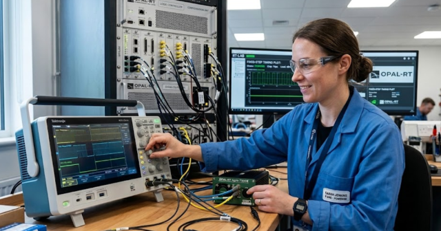
Set up SIL runs and automation using RT-LAB workflows
SIL delivers value when runs are automated, comparable, and easy to reproduce across builds. A consistent workflow compiles models into deterministic executables, loads test vectors, and collects results into a single format your team trusts. RT-LAB is often used to manage this run lifecycle, including parameter sweeps and data logging. Automation keeps “works on my machine” out of validation.
A solid setup starts with versioned models, versioned test cases, and a clear naming scheme for outputs. Test automation should reset initial conditions the same way every time, then assert pass fail criteria that match your engineering intent. Logging should capture both the stimulus and the controller response, plus timestamps, so regressions are obvious. You’ll also want a lightweight way to rerun a failing case locally without rebuilding the whole test bench.
Execution context matters here, not vendor claims. Teams using RT-LAB within OPAL-RT setups typically standardize compilation targets, sample times, and logging templates so engineers can focus on control intent instead of run mechanics. That kind of standardization pays off when a late bug appears and you need to prove when it was introduced. The goal is a paper trail of results that stays consistent across weeks, not heroic debugging sessions.
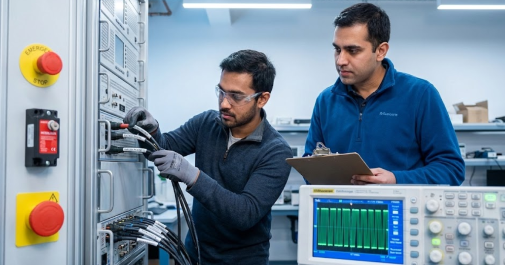
Configure HIL hardware I/O signal conditioning and safety interlocks
HIL testing succeeds when I/O is engineered like a product, not wired like a prototype. Map every input and output with ranges, scaling, and timing expectations, then verify that the simulator, I/O modules, and controller all agree. Add signal conditioning so your controller sees realistic voltages, currents, and encoder patterns. Safety interlocks must always win over test convenience.
A practical setup could pair an inverter controller with analog current feedback, resolver inputs, discrete gate-disable lines, and a CAN command interface, then route those through appropriate isolation and scaling so fault conditions stay bounded. That single rig forces you to validate details SIL cannot, such as what happens when an analog channel saturates, a discrete line chatters, or a bus message arrives late. It also forces clear ownership of who can arm outputs, who can clear faults, and what the safe state is after a stop. Those are engineering choices, not wiring trivia.
Interlocks should be layered. Hardware e-stops, watchdogs, and output inhibit logic should act even if the host PC freezes, and your test scripts should never be the only guardrail. Treat every connector and pinout change as a configuration item, since accidental mis-scaling can look like a control defect. Your fastest path to trustworthy results is tight I/O discipline and a safety plan that never relies on hope.
Tune real-time performance with solvers step size and FPGA
Real-time performance is the ability to finish each simulation step on time, every time, while keeping numerical behaviour stable. Step size choices set the ceiling for what dynamics you can represent and how accurately you can emulate timing. Solver selection, model partitioning, and I/O scheduling decide if you hit deadlines without jitter. FPGA resources matter when sub-millisecond determinism and high-rate I/O are mandatory.
Start with the control loop requirements, then work backward into the plant fidelity needed to make the same control decision. If the plant model forces a smaller step than your compute target can sustain, reduce stiffness, simplify switching detail, or move the tightest parts onto FPGA. Keep an eye on the full loop, since fast analog I/O, encoder decoding, and bus stacks all compete for time. Determinism is the metric that matters, because occasional overruns make fault logic look random.
Performance tuning should stay transparent. Track step execution time, jitter, and dropped frames as first-class test outputs, not hidden diagnostics. Partitioning decisions should be documented so a later model update does not silently move work onto the CPU and break timing. Once timing is stable, lock key settings, then treat changes as controlled experiments with measurable impact.
Create repeatable test cases fault injection and result reviews

Repeatable test cases turn HIL and SIL from demos into validation evidence. Each case should declare initial conditions, input stimuli, expected outputs, and explicit tolerances, then store results so comparisons are meaningful across builds. Fault injection belongs here, because electrified controllers are judged heavily on how they fail. Result reviews should focus on trends and regressions, not one-off plots.
Good fault injection is specific and bounded. Inject sensor bias, stuck-at values, bus timeouts, and actuator disable events at precise times, then verify the controller transitions through the expected states without unsafe outputs. Pair these checks with clear acceptance rules so teams stop arguing about what “looks fine” means. Store the exact model version and parameter set for every run, because calibration drift can masquerade as logic drift.
Discipline is the differentiator over time. Teams that treat tests as code, review changes, and keep baselines clean will ship with fewer late surprises than teams that chase ad hoc failures. OPAL-RT fits best when it supports that discipline through repeatable execution and traceable results, not when it’s treated as a one-time lab purchase. Confidence comes from consistent proof, and consistent proof comes from controlling the details you can control.
Real-time solutions across every sector
Explore how OPAL-RT is transforming the world’s most advanced sectors.
Industry applications, Simulation
03 / 31 / 2026
Managing high-frequency switching in real-time EMT simulation
Precision in testing complex power systems is essential to avoid failures, accelerate innovation, and integrate new technologies safely.

Simulation
03 / 30 / 2026
Understanding timestep requirements for modern power converters
Practical criteria for selecting EMT and real time simulation timesteps for power converters, covering switching resolution, control and PWM timing alignment, multirate approaches, and verification checks.

Energy, Industry applications, Simulation
03 / 29 / 2026
Validating data center energy management systems using real-time HIL
This piece explains how AI workload variability affects data centre power stability and how closed-loop HIL testing helps validate EMS control behaviour under site and grid stress.
EXata CPS has been specifically designed for real-time performance to allow studies of cyberattacks on power systems through the Communication Network layer of any size and connecting to any number of equipment for HIL and PHIL simulations. This is a discrete event simulation toolkit that considers all the inherent physics-based properties that will affect how the network (either wired or wireless) behaves.