Understanding timestep requirements for modern power converters
Simulation
03 / 30 / 2026

Key Takeaways
- Treat timestep as a verifiable requirement tied to what you must measure, not a default solver setting.
- Align plant, PWM, and control timing so delay and jitter stay deterministic and test results stay comparable.
- Use multirate or averaged models when switching detail exceeds your real time compute budget, then confirm correctness with convergence and spectral checks.
You’ll pick the right power converter simulation timestep by treating it as a system requirement, not a solver preference.
“Modern converters keep pushing switching edges faster, control loops tighter, and protection actions more time-sensitive, so a default timestep will fail you sooner than you expect.”
Wide bandgap semiconductors are cited as supporting up to 10× higher switching frequencies than silicon, which forces smaller steps if you want switching behaviour you can trust. The practical stance is simple: choose a timestep from the signals you must resolve, then prove it with checks that catch aliasing, timing slip, and numerical artefacts.
Start from switching frequency and required time resolution
The timestep must be short enough to resolve the switching period and the edge-related dynamics you care about, such as ripple, harmonic content, and device stress proxies. If the step is too large, switching events collapse into a smeared average and your results look stable but won’t match measurements. A good starting point is to target many solver steps per switching period, then tighten only when a specific metric fails.
Start with the question you’re actually trying to answer. If you need current ripple for capacitor sizing, common-mode voltage for insulation stress, or high-frequency content for EMI filters, you need a step that lands predictably around PWM transitions. If you only need average torque, bus voltage regulation, or thermal trends, you can often relax the step and move the switching detail into an averaged representation.
Also decide which timing errors are acceptable. A small error in average current might be fine, while a small error in protection timing can be unacceptable because it changes trip sequencing. Timestep selection gets easier when you set pass or fail criteria first, then you tune the step until those criteria stop moving.
Link timestep to control loops, PWM, and measurement delays
Your electrical timestep and your control timing must line up, or the simulator will create artificial delay and jitter. PWM updates, sampling instants, and sensor filtering all happen on discrete schedules, and your simulation step acts like the clock that decides when those schedules advance. If that clock is poorly chosen, the controller can look slower or faster than it really is.
Map the timing chain end-to-end. Start at the ADC sampling point, add digital filtering and computation time, then include PWM update timing and any intentional deadtime. Each element adds delay, and delay changes phase margin. A controller that is stable on paper can ring or even become unstable in simulation if the effective delay shifts by even a fraction of a sample.
Make the ordering deterministic. You want a consistent sequence such as measure, compute, update duty, then apply switching in the plant. If the plant step and the control step are not harmonized, the controller will act on stale data or apply a duty change half a step late, and you’ll waste time chasing a “control problem” that is really a timing problem.
Balance accuracy, stability, and runtime cost in EMT models
Electromagnetic transient models trade time resolution for numerical stiffness and compute load, so the best timestep is the smallest one that passes your accuracy checks with stable behaviour. Too large a step distorts switching harmonics and transient peaks. Too small a step can amplify numerical noise, stress solver tolerances, and blow your real time budget, even if the physics would be fine.
Aliasing is the quiet failure mode that misleads teams, because the waveform still looks “clean.” Sampling theory states the sampling rate must be at least 2× the highest frequency component you want to represent, or higher-frequency content folds into lower-frequency results. Switching edges contain energy well above the carrier, so you will treat the timestep as a bandwidth limiter, not just a numerical knob.
| What you need to trust | What timestep pressure looks like | What you can do if pressure is too high |
| Average power flow and DC bus regulation | Larger steps still match means but hide ripple | Use an averaged switch model and validate means |
| Switching ripple used for passive sizing | Steps that are too large understate RMS ripple | Increase steps per switching period until ripple converges |
| Harmonics used for grid or filter compliance checks | Aliasing shifts spectral content into the wrong bands | Reduce timestep or isolate switching in a faster submodel |
| Protection timing and fault transients | Event timing slips and peak currents get clipped | Use smaller steps during faults or event-triggered refinement |
| Closed-loop stability margins and damping | Artificial delay appears through sample misalignment | Align control and plant rates and keep delay accounting explicit |
Choose a real-time EMT timestep under hardware limits
“Timestep problems show up as results that look plausible but shift when you change the step, reorder tasks, or modify logging.”
A real-time EMT timestep must satisfy physics and still complete within the fixed compute budget of each step. That constraint turns timestep selection into an engineering contract: fidelity must fit into the available CPU and FPGA cycles, plus I/O latencies, with enough headroom for worst-case events like faults. If you miss the deadline, the run stops being real-time and your closed-loop test loses meaning.
Consider a three-phase, two-level inverter running 20 kHz PWM with a current controller sampled at 10 kHz, connected to a plant model that includes an LCL filter and a stiff grid source. A practical starting point is to choose a plant timestep that gives solid resolution inside each switching period, then set the control to execute on an integer multiple of that step so the sample, compute, and PWM update happen on repeatable boundaries. After that, tighten the timestep only if ripple, harmonics, or protection timing fails your acceptance checks.
Execution details matter as much as the number. OPAL-RT real-time digital simulators are typically configured so you can pin fast, repetitive switching computations to deterministic resources and keep slower network, thermal, or supervisory functions at a larger step. That split keeps your real-time EMT timestep honest without forcing the whole model to run at the fastest rate.
Use multirate and averaged models for very fast switches
Multirate and averaged modelling protect you from chasing nanoseconds with a full-system EMT step. When switching edges become far faster than the electrical time constants you care about, pushing the entire model to a tiny timestep wastes compute and often makes validation harder. A better approach is to keep the system step aligned to the dynamics of interest and represent switching detail only where it affects your acceptance metrics.
Multirate simulation assigns a small step to a limited subnetwork, such as the converter bridge and its nearest parasitics, while the rest of the grid or machine runs at a larger step. Averaged models replace the discrete switch with a duty-cycle controlled source, so you preserve control-to-output dynamics and power balance without resolving every transition. Hybrid approaches also work well, running averaged behaviour during steady-state and switching detail during specific transient windows you care about.
The key tradeoff is observability. Averaged models will not give you switching ripple or high-frequency spectra, so they only belong in tests where those quantities are out of scope. When you need both system-scale behaviour and switching details, multirate is usually the cleaner choice than shrinking the global timestep until the platform breaks.
Spot timestep problems using waveforms, spectra, and convergence checks
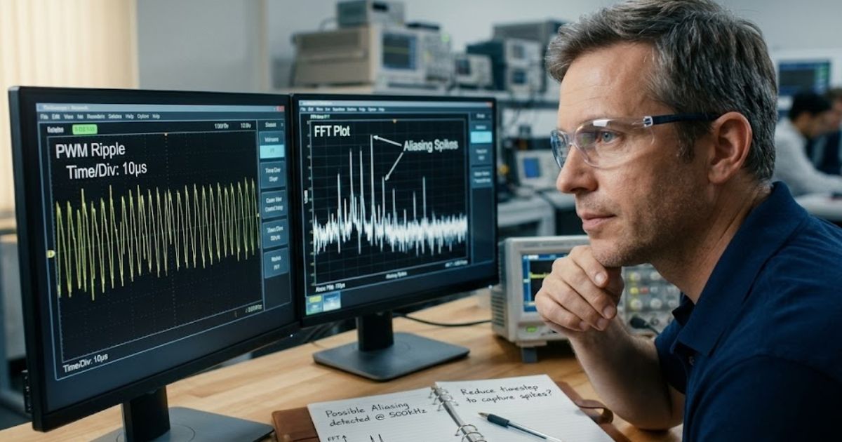
Timestep problems show up as results that look plausible but shift when you change the step, reorder tasks, or modify logging. You’ll catch them faster with a small set of repeatable checks that test timing, spectrum, and convergence, rather than relying on a single waveform screenshot. If the check fails, treat the timestep as the first suspect before you re-tune control gains.
- Halve the timestep and confirm key metrics change minimally
- Compare duty updates against PWM carrier boundaries for jitter
- Check ripple RMS and peak values over identical windows
- Run an FFT to spot aliasing and missing switching bands
- Trigger a fault and confirm protection timing stays consistent
Good checks also protect your team from accidental regression. Logging decimation, control task scheduling, and I/O buffering can all hide timing errors until you close the loop with hardware and the mismatch becomes expensive. The most reliable workflow keeps a small set of “golden” runs and requires convergence on the quantities you actually sign off, not on every internal state.
Discipline is the differentiator. Teams that treat timestep as a measurable requirement get stable models, predictable tests, and clean handoffs across control, power, and test engineering. OPAL-RT fits best when you use that discipline to lock timing, validate convergence, and keep real-time execution aligned to the converter’s true switching and control behaviour.
Real-time solutions across every sector
Explore how OPAL-RT is transforming the world’s most advanced sectors.
Industry applications, Simulation
03 / 31 / 2026
Managing high-frequency switching in real-time EMT simulation
Precision in testing complex power systems is essential to avoid failures, accelerate innovation, and integrate new technologies safely.

Industry applications, Simulation, Energy
03 / 29 / 2026
Validating data center energy management systems using real-time HIL
This piece explains how AI workload variability affects data centre power stability and how closed-loop HIL testing helps validate EMS control behaviour under site and grid stress.

Industry applications
03 / 28 / 2026
Control algorithm validation using real-time HIL
A practical look at how real-time HIL testing validates embedded control algorithms through closed-loop simulation, fault reproduction, digital plant models, and disciplined integration.
EXata CPS has been specifically designed for real-time performance to allow studies of cyberattacks on power systems through the Communication Network layer of any size and connecting to any number of equipment for HIL and PHIL simulations. This is a discrete event simulation toolkit that considers all the inherent physics-based properties that will affect how the network (either wired or wireless) behaves.