CPU versus FPGA simulation for high speed motor drive testing
Simulation
02 / 26 / 2026
Key Takeaways
- Pick CPU simulation when your HIL goals tolerate larger fixed steps and consistent I/O delay, and your pass criteria focus on control logic and averaged electrical behaviour.
- Require FPGA simulation when your tests depend on switching edges, microsecond timing, and deterministic protection response that a CPU cannot guarantee under worst-case load.
- Lock your choice with measurable acceptance criteria for step size, overrun margin, and end-to-end I/O latency, then match model fidelity to the faults you must sign off.
Choose CPU simulation until microsecond timing becomes a hard test requirement.
High speed motor drive testing breaks when your simulator smooths away the very events that trip protection, saturate current sensors, or destabilize a fast current loop. Electric motors account for about, so getting drive behaviour right matters well beyond a single controller project.
CPU vs FPGA simulation is not a spec-sheet contest.
The practical separator is timing certainty at the step size you need, plus I/O latency that stays predictable when the loop is closed through hardware in the loop (HIL). Start from your test goals, write acceptance criteria, and pick the simplest compute that will meet them every time.
Choose CPU or FPGA based on motor drive HIL goals
The main difference between CPU and FPGA simulation is how they handle time and concurrency in real-time execution. A CPU runs sequential code very fast but still fights scheduling jitter and step-size limits. An FPGA runs many operations in parallel with deterministic timing, which matters when your test depends on sub-cycle switching behaviour.
CPU-based HIL fits best when you’re validating control logic, startup sequences, fault state machines, and monitoring that depends on averaged electrical behaviour. FPGA-based HIL fits best when you must represent switching edges, dead time effects, and fast protection paths without hiding them inside a large time step. A mixed approach also works well when only the power stage needs microsecond resolution.
| What you must capture in HIL | Compute choice that usually fits |
| Control behavior at millisecond and tens of microseconds time scales. | CPU simulation with a fixed-step solver. |
| Switching ripple and transient currents tied to PWM edges. | FPGA simulation with microsecond steps. |
| Very low and repeatable I/O latency for closed-loop protection. | FPGA-based I/O and plant partitioning. |
| Large plant scope where model size matters more than switching detail. | CPU simulation with simplified power stage models. |
| Mixed fidelity where the inverter is detailed but mechanics stay coarse. | Hybrid CPU and FPGA split across subsystems. |
Know the timing limits that break CPU-based simulation
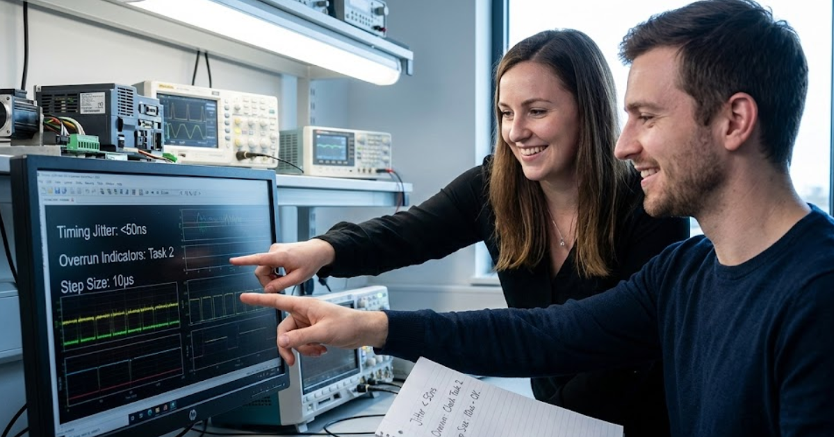
CPU simulation breaks down when your required fixed time step gets so small that the solver and I/O tasks cannot finish before the next tick. Missed deadlines show up as overruns, jitter, or forced step-size increases, and those artifacts will corrupt the same measurements you use to judge controller quality.
Timing risk rises when you pile switching models, sensor filtering, and interface handling into the same loop. A faster CPU helps, but determinism still depends on worst-case execution time, not average performance. Multi-core setups can also surprise you if threads contend for memory or if I/O handling steals cycles at the wrong moment.
Practical acceptance starts with a hard time budget: plant solve time plus I/O sampling, plus any logging, plus safety margin. If your tests require single-digit microsecond steps and tight loop closure to physical controllers, a CPU-only approach turns into a constant fight against margin. When the needed step is looser, CPU simulation stays productive and easier to iterate.
Use FPGA simulation for switching level power electronics fidelity
FPGA simulation is required when switching-level fidelity is the test, not a detail you can average away. Deterministic parallel execution lets you represent device-level behaviour, PWM timing, and fast protection paths at very small time steps. That fidelity keeps faults, ripple, and commutation effects visible to the controller.
Higher switching frequencies push you toward that approach because the electrical system changes more within each control period. Wide bandgap semiconductors can support switching frequencies up to 10 times higher than silicon devices, which tightens timing requirements for any test that cares about current ripple, dv/dt-related effects, or cycle-by-cycle protection.
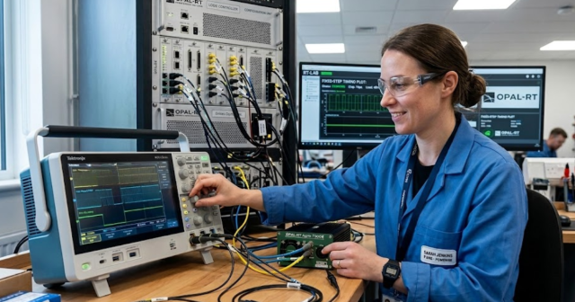
FPGA work does add constraints. Model development often uses fixed-point arithmetic, careful scaling, and explicit partitioning between what must run at microseconds and what can run slower. Platforms such as OPAL-RT are commonly used to split CPU and FPGA workloads cleanly, so you keep fast power stage timing deterministic while leaving supervisory logic and larger system context on the CPU.
Match solver step size to PWM frequency and control loops
Step size selection should start from the fastest phenomenon your test must observe, then work backward to what the controller will do with that information. If you only need average torque and speed response, you can run larger steps and simplify switching. If you need cycle-by-cycle behaviour, step size must be small enough to preserve it.
A concrete check helps: a 20 kHz PWM period is 50 µs, and a current loop can run at several kHz on top of it. Using a 25 µs plant step will leave you with only two points per switching period, which will smear switching ripple and can hide the peak current that triggers protection. A 1 µs to 2 µs step resolves far more of the switching period and keeps peak behaviour visible to both software and hardware fault logic.
Solver choice and partitioning matter as much as the raw step size. Averaged inverter models can be valid for control tuning and efficiency studies, but they will not validate gate timing, dead time compensation, or cycle-accurate desaturation paths. Switching models also require you to treat sampling, quantization, and delay as first-class parts of the test, not as afterthoughts.
Check I/O latency and interface needs for motor drive testing
I/O latency is part of the plant when you close the loop through HIL. The controller reacts to measured currents, voltages, and position, and it expects those signals to arrive with stable delay. If that delay moves around, tuning results won’t carry over and protection validation loses credibility.
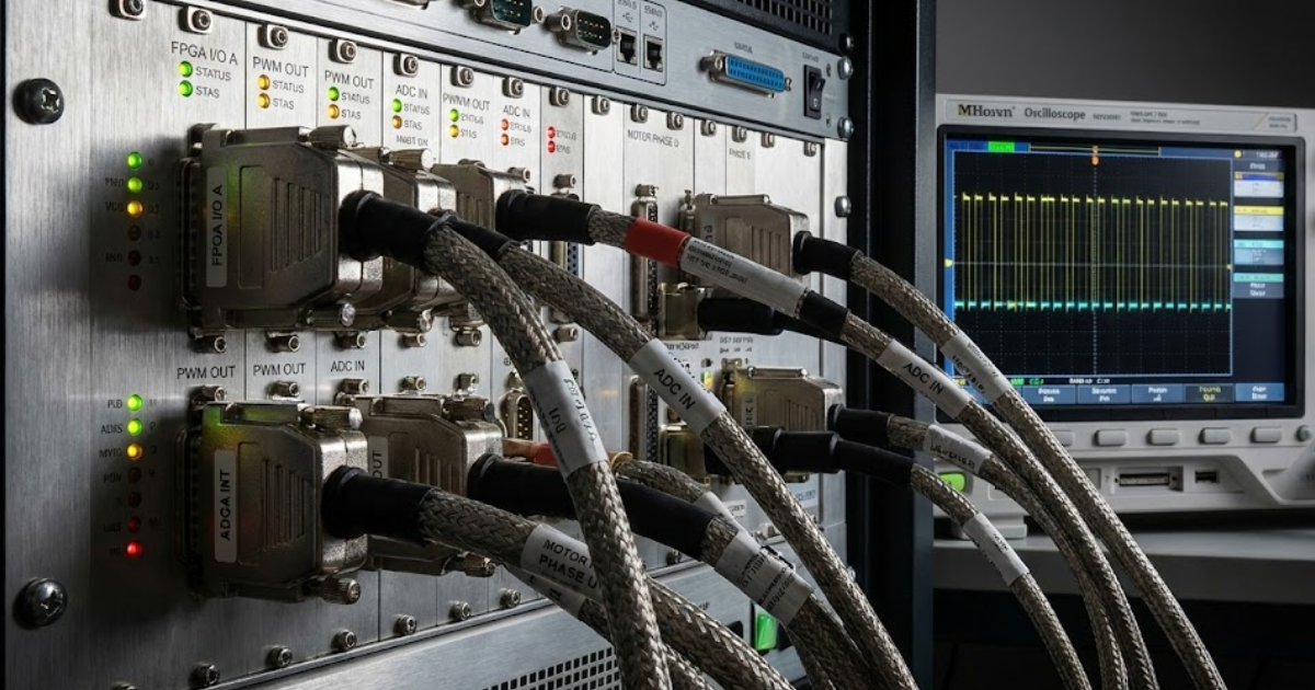
Start with the interfaces your controller actually uses: PWM outputs, gate commands, current feedback, DC link sensing, encoder or resolver position, and fault lines. Each signal path adds conversion time, buffering, and scheduling overhead, and the total must stay inside your loop budget. Deterministic latency often matters more than minimum latency because a consistent delay can be compensated, while jitter turns into phase noise.
Hardware partitioning is a timing tool, not just a compute tool. Fast I/O capture and generation pairs naturally with FPGA execution when you need a repeatable microsecond-scale response. CPU execution fits when your interfaces are slower, your control periods are longer, or your main goal is functional behaviour rather than edge-level timing.
Avoid common selection mistakes and set clear acceptance criteria
The common mistake is choosing compute first and test intent second. CPU-only setups fail when teams assume average performance equals deterministic performance, or when they ask a large plant model to run at microsecond steps. FPGA-only setups fail when teams spend time on switching detail that the test plan never uses.
Write acceptance criteria that are measurable during commissioning, then hold the setup to them. Keep criteria tied to your controller’s actual sampling and protection paths, not to general simulator performance claims. Align the model detail to the fault cases you must sign off, and strip everything else back to what supports those cases.
- Your fixed time step will stay stable under worst-case fault scenarios.
- End-to-end I/O delay will be repeatable within your loop budget.
- Switching detail will appear only when your test needs it.
- Overruns and jitter will be logged and treated as test failures.
- Model scope will match the signoff questions, not team preferences.
CPU vs FPGA simulation stops being a debate when you treat timing and latency as engineering requirements.
Choose CPU when it meets the step size and I/O stability you can prove during HIL checkout, and choose FPGA when switching-level dynamics and deterministic response are part of the pass criteria. Teams that execute this discipline on OPAL-RT platforms tend to move faster in the lab because the simulator choice is anchored to measurable behaviour, not to assumptions.
Real-time solutions across every sector
Explore how OPAL-RT is transforming the world’s most advanced sectors.
Industry applications, Simulation
03 / 31 / 2026
Managing high-frequency switching in real-time EMT simulation
Precision in testing complex power systems is essential to avoid failures, accelerate innovation, and integrate new technologies safely.

Simulation
03 / 30 / 2026
Understanding timestep requirements for modern power converters
Practical criteria for selecting EMT and real time simulation timesteps for power converters, covering switching resolution, control and PWM timing alignment, multirate approaches, and verification checks.
Energy, Industry applications, Simulation
03 / 29 / 2026
Validating data center energy management systems using real-time HIL
This piece explains how AI workload variability affects data centre power stability and how closed-loop HIL testing helps validate EMS control behaviour under site and grid stress.
EXata CPS has been specifically designed for real-time performance to allow studies of cyberattacks on power systems through the Communication Network layer of any size and connecting to any number of equipment for HIL and PHIL simulations. This is a discrete event simulation toolkit that considers all the inherent physics-based properties that will affect how the network (either wired or wireless) behaves.