How to scale power validation from 5 to 30 kW using modular PHIL systems
Power Systems
04 / 14 / 2026

Key Takeaways
- Stable PHIL scaling starts with loop delay, impedance, and interface design, because extra kilowatts only help after the feedback path is proven.
- Matched power blocks scale better than mixed hardware because repeated control, sensing, and protection logic cut recommissioning work.
- A 10 kW building block gives labs a practical path from bench validation to 30 kW without rewriting methods for every new test range.
Scaling power validation from 5 kW to 30 kW works when you scale loop control, protection, and interface design before you add amplifier modules.
Global electric car sales exceeded 17 million in 2024. That volume keeps pushing charger, inverter, and battery subsystems into mid-power validation sooner. A modular PHIL setup lets you add power in blocks while keeping the same model, interface logic, and safety plan. You won’t get stable 30 kW results by stacking amplifiers and hoping the feedback loop holds.
Scaling PHIL power starts with loop stability limits
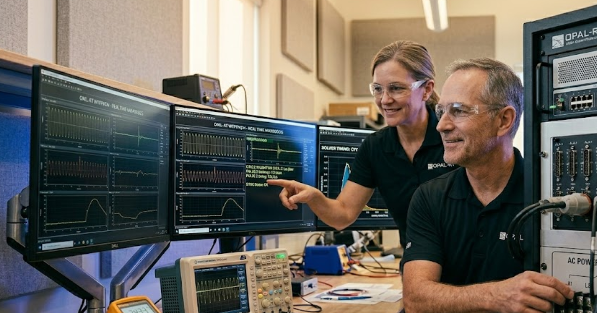
Scaling from 5 kW to 30 kW starts with loop stability because the closed loop will fail before the amplifier reaches its nameplate limit. Delay, impedance mismatch, and interface algorithm choice set the usable power ceiling. Once those terms are controlled, higher power becomes repeatable rather than fragile.
Consider a 5 kW motor drive tied to a virtual grid through an interface with comfortable phase margin. That same device can oscillate at 20 kW during a step load even though the hardware still has thermal headroom. Extra current magnifies phase error, and the first sign is often noisy sharing or a voltage overshoot that looks like a hardware fault. You’re facing a loop problem that a larger cabinet will not fix.
You should check small signal stability, interface delay, and source impedance before planning added modules. Teams that skip that order usually retune protection after every power step, which slows commissioning and muddies test results. A stable 5 kW setup gives you the template for 10, 20, and 30 kW only when the closed-loop math stays consistent. That discipline saves time later because the next power increment becomes a verification task instead of a rescue task.
“Scaling from 5 kW to 30 kW starts with loop stability because the closed loop will fail before the amplifier reaches its nameplate limit.”
A modular PHIL system scales through matched power blocks
A modular PHIL system scales cleanly when each power block behaves like the same electrical and control element. Matched voltage ranges, identical sensing chains, synchronized clocks, and the same protection logic keep one added block from becoming a new commissioning exercise. Repetition is what makes added power usable.
A practical pattern is three 10 kW regenerative amplifiers wired as one 30 kW stage. Each block sees the same reference, the same current feedback path, and the same fault logic, so you only validate one unit thoroughly. When the third block is added, your model interface and test scripts stay intact. You’re extending a verified cell rather than rebuilding the rig.
Mixed blocks are where trouble starts. Pairing a fast module with a slower one can skew current sharing during transients, and a different sensor range can distort calibration under the same command. You’ll get better scale and cleaner data from matched modules than from a pile of available hardware that happens to add up to 30 kW. That is the practical meaning of modularity in PHIL.
A modular power supply unit does not define scalability
A modular power supply unit does not automatically scale PHIL because modularity means different things in different hardware categories. A fully modular power supply can refer to removable cables, and a modular PC power supply serves computer assembly needs. PHIL needs bidirectional power flow, bandwidth, and tight closed-loop control.
That distinction matters when teams search for a modular power supply and assume any stackable source will work for power hardware in the loop. A bench supply with neat cable management can power control boards just fine, yet it can’t reproduce grid impedance or sink returned energy from a motor inverter. The label sounds similar, but the test job is completely different. Your selection criteria have to follow the loop and the power interface.
The same confusion shows up with modular versus non-modular power supply comparisons. Cable modularity affects serviceability and airflow in electronics enclosures, while PHIL modularity affects current sharing, stability, and protection behaviour under feedback. Once you separate those ideas, hardware choices get far clearer. You stop shopping for convenience features and start validating the properties that make closed-loop tests credible.
The power interface matters more than nameplate kilowatts
The power interface determines how the simulator and hardware exchange energy, so it sets accuracy and stability more directly than the kilowatt rating on the rack. Interface choice shapes phase margin, transient fidelity, and fault behaviour. A bigger amplifier will not repair a weak interface.
Two 30 kW systems can behave very differently during the same inverter test. One setup using a damping impedance method can stay calm during a line disturbance, while another using a poorly tuned ideal transformer approach can ring and trip on the same event. You can see the difference during voltage sags, harmonic injection, or rapid current reversals. The rating sheet looks identical, yet the usable test envelope does not.
Choose the interface around the device under test and the fault cases you need to run. Grid-tied converters often need a different interface emphasis than battery emulators or motor drives. Once the interface is right, the power stage becomes easier to duplicate because the control assumptions stay stable. That is why interface work belongs near the start of a scaling plan.
| Checkpoint | What it tells you before you add power |
|---|---|
| Closed-loop delay | If delay already erodes phase margin at 5 kW, extra modules will multiply error during current steps. |
| Interface algorithm | The wrong interface can look calm at light load and fail once source impedance and transient energy rise. |
| Current sharing method | Parallel blocks need one reference and matched sensing or one module will absorb most of the surge. |
| Protection zoning | Isolation and trip logic must clear faults without collapsing the whole test or erasing useful traces. |
| Expansion block size | Repeating one validated power block cuts recommissioning work and preserves comparable results across programmes. |
Parallel modules work only with tight timing control
Parallel power modules only behave as one source when timing stays tightly aligned across control loops, sensing, and switching updates. Even small skews will push one module to lead and another to lag during transients. Clean current sharing depends on synchronized timing first and firmware tuning second.
A three-module setup can look fine at steady state and still misbehave during a 0% to 100% load step. One block grabs the surge, hits its current limit, and forces the other two into recovery. That sequence usually starts with sample skew or mismatched filters rather than bad hardware. OPAL-RT users often handle this by tying simulator timing, analogue I/O, and amplifier commands to one deterministic schedule before they raise power.
You’ll want to verify timing at the boundaries where modules interact, not only inside the simulator. Sensor latency, networked command updates, and output filter differences all matter once blocks are paralleled. Tight timing control is the reason a modular rig feels like one instrument instead of three separate sources sharing a bus. That single behaviour model is what lets a lab trust fast transients.
Protection design sets the safe path to 30 kW
Protection design sets the safe path to 30 kW because fault energy rises faster than most labs expect when extra modules are added. Trip settings, isolation strategy, and fault containment have to scale with the bus, not just with each amplifier. Safety logic must remain selective under feedback.
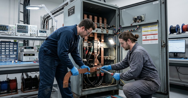
Consider a regenerative inverter test that is calm at 5 kW but throws a hard current reversal during a controller fault. A single global trip will shut the whole rig down and erase the trace you need, while badly coordinated local trips can leave the bus in an undefined state. You need layered protection that isolates the failing branch and preserves the rest of the measurement chain long enough to capture what happened. That is how safety and useful data stay aligned.
- Set fast overcurrent limits for each module and for the shared bus.
- Separate local trips from full system shutdown logic.
- Verify contactor timing against worst-case regenerative energy.
- Match fuse and breaker clearing behaviour to your fault study.
- Record pre-trip signals so protection events stay diagnosable.
Those checks save time during commissioning because they turn protection from guesswork into an engineered sequence. You’re also protecting test credibility. A lab that trips cleanly and records the event will scale faster than a lab that resets blindly after every fault. Safe expansion is a control problem as much as a power problem.
Modular versus fixed power hardware affects lab cost
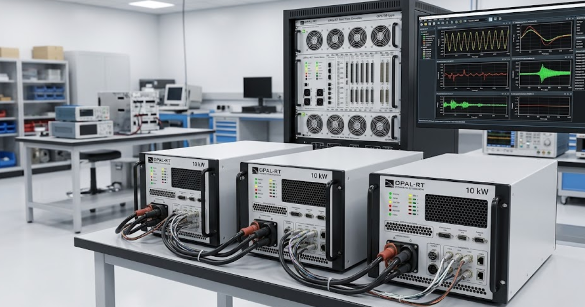
The main difference between modular and fixed power hardware is that modular hardware spreads cost across repeated test blocks, while fixed hardware concentrates cost in one larger unit with fewer integration variables. Your best option depends on how often test power, topology, and lab use cases shift over time.
A fixed 30 kW source can make sense for one stable programme with narrow operating modes. Commissioning is often shorter because fewer internal sharing loops exist. A modular setup suits labs that move between charger emulation, inverter validation, and grid disturbance tests, since the same blocks can be reassigned or partially deployed. That flexibility matters when one bench needs 10 kW this month and 30 kW later.
“A repeatable 10 kW block makes expansion planning practical because it matches many mid-power validation tasks and stacks cleanly to 20 or 30 kW without rewriting your lab method.”
Cost should be judged across reuse, downtime, spare strategy, and recommissioning labour. A non modular power supply can look cheaper on a quote and cost more after a topology shift forces new protection work or leaves half the rack idle. Modular hardware earns its keep when your test plan refuses to stay still. You’re paying for repeatable reuse, not just for rated output.
A repeatable 10 kW block simplifies expansion planning
A repeatable 10 kW block makes expansion planning practical because it matches many mid-power validation tasks and stacks cleanly to 20 or 30 kW without rewriting your lab method. Public charging guidance places Level 2 hardware at 3 to 19.2 kW and direct current fast charging at 50 to 350 kW.
That spread explains why 10 kW is such a useful planning unit. One block covers onboard chargers, smaller inverters, and battery interface tests. Three blocks can support a 30 kW bench with the same wiring philosophy, calibration routine, and protection map. You’re building a habit of repetition, which is what makes higher power feel controlled rather than improvised.
Teams that scale well treat every added module as a copy of proven behaviour. OPAL-RT fits that discipline when the simulator, I/O, and power hardware are commissioned as one timed system instead of separate purchases. That approach gives you a lab that produces comparable results at 5, 10, and 30 kW, which is what careful validation is supposed to do. Good scaling feels calm because the method stays the same as the power rises.
Real-time solutions across every sector
Explore how OPAL-RT is transforming the world’s most advanced sectors.
Microgrid
09 / 19 / 2026
Hybrid AC-DC microgrid emulation with power hardware-in-the-loop
An examination of how hybrid AC-DC microgrid stability is set at the interlinking converter and why power hardware in the loop is required to test that boundary at full power.

Power Electronics
09 / 17 / 2026
BLDC motor control fundamentals with simulation examples
A technical primer on six step BLDC commutation, Hall sensor and sensorless back EMF position sensing, torque ripple at each switching instant, and the simulation exercises a teaching lab can run.

Power Systems
09 / 16 / 2026
How to build a protection relay testing workflow utility engineers trust
A practical look at how utility engineers build protection relay testing workflows, from secondary injection through closed loop validation against a real time power system model.