9 Common hardware in the loop testing pitfalls in embedded and control validation
Simulation
03 / 11 / 2026
Key Takeaways
- Run HIL testing only after you’ve proven deterministic timing, including worst-case loop delay and jitter under load.
- Match plant model fidelity, solver choices, and sensor actuator non-idealities to what the controller is sensitive to, not to what looks good on plots.
- Protect test credibility with disciplined integration controls such as consistent signal contracts, automated repeatable runs, and strict version traceability.
Most HIL testing failures don’t come from one big mistake. They come from small mismatches that compound across timing, model fidelity, and integration details until the test rig becomes hard to trust. When that happens, teams either overcorrect with expensive lab work or ship with gaps they thought HIL had covered.
A disciplined hardware in the loop simulation setup prevents that spiral. You don’t need perfection everywhere, but you do need to know what must be accurate, what can be approximate, and how to prove the difference with repeatable checks. The pitfalls below focus on the failure modes that most often break embedded and control validation.
“Hardware in the loop testing only builds confidence when timing, models, and interfaces match your target.”
Set clear HIL test goals before wiring anything
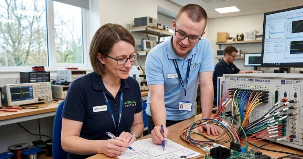
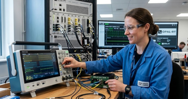
Hardware in the loop connects your real controller to a simulated plant so you can test closed-loop behaviour safely and repeatably. The fastest path to reliable results starts with a written target for timing, interfaces, and acceptance criteria, because those choices determine model fidelity, I/O hardware, and how you interpret every pass or fail.
Define what “good” means before anyone debates tooling or model detail. That simple step prevents teams from “tuning the rig” to get the answer they want, instead of validating the control system they actually plan to ship.
- Control bandwidth and sample time targets
- I/O ranges, loads, and isolation needs
- Network protocols and timing tolerances
- Pass fail criteria tied to requirements
- Traceability for models and test scripts
9 hardware in the loop testing pitfalls and fixes
Common problems with hardware in the loop testing cluster into three themes: timing that isn’t deterministic, models that don’t represent what the controller “feels,” and integrations that quietly distort signals. Treat each pitfall as a checkpoint you can verify early, before you scale up test coverage or start chasing controller bugs.
1. Timing budgets missed from step size and I/O latency
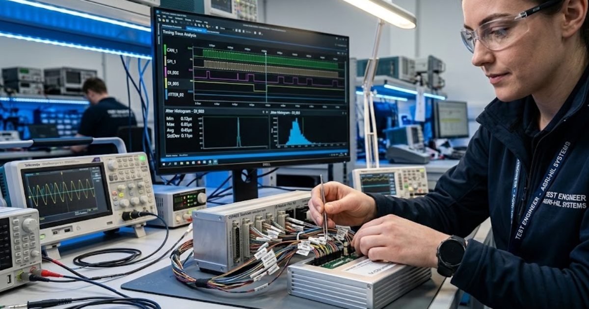
HIL simulations fail in embedded systems when the controller’s expected sample timing doesn’t match the simulator’s step size plus I/O and driver latency. Fix this by treating timing as a budget you measure, not a setting you assume. Lock a fixed-step schedule, then confirm end-to-end loop delay and jitter under load.
Latency hides in places teams overlook: ADC and DAC conversions, protocol stacks, and host CPU contention. A real-time execution trace should show the worst-case step overrun and the worst-case I/O update age, not only an average. When you use platforms such as OPAL-RT, rely on deterministic scheduling and instrumentation to prove the timing budget stays inside your controller’s tolerance.
2. Plant model fidelity too low for controller bandwidth
A plant model that looks stable at low frequency can be useless at the controller’s bandwidth, where delays, resonances, and saturation shape stability margins. Fix this by matching model fidelity to the control objective, then validating the model response at the frequencies the controller will excite. Keep high-frequency dynamics that affect phase and gain.
Fidelity is not the same as complexity. You can often remove slow thermal or mechanical detail while preserving the fast electrical or hydraulic dynamics that dominate closed-loop behaviour. A practical check is a frequency response or step response comparison against a trusted baseline, then a quick sensitivity run to see which parameters move your pass or fail outcomes.
3. Solver and discretization choices create aliasing and instability
Solver settings can add energy, erase damping, or alias switching effects into fake oscillations. Fix this by selecting solvers and discretization that match your plant physics and your real-time step, then verifying numerical stability with stress cases. Sampling too slowly turns legitimate high-frequency content into misleading low-frequency behaviour.
Aliasing often shows up as “controller instability” that disappears on the bench. Pay attention to discontinuities, switching events, and transport delays, then choose modelling approaches that behave predictably under fixed-step execution. When the plant includes fast switching or stiff dynamics, a smaller step size, solver changes, or dedicated computation paths will be required to keep the simulation consistent.
4. Signal scaling and electrical conditioning errors corrupt measurements
Incorrect scaling and conditioning quietly ruin results because the controller still runs and your plots still look plausible. Fix this with a strict signal contract for every channel: units, scaling, polarity, offset, filtering, and expected noise. Confirm the contract with loopback checks and known injected values before running complex scenarios.
Electrical details matter as much as math. Input impedance, sensor excitation, isolation, grounding, and common-mode limits can distort measurements or trip protections. If your HIL rig uses signal conditioning, treat it like part of the plant, because it changes what the controller “sees.” A clean calibration record for each channel will save days of debugging later.
5. Protocol integration hides jitter, packet loss, and retries
Networked I/O can look fine functionally while failing temporally, especially when retries and buffering mask missed deadlines. Fix this by measuring message age, jitter, and loss under worst-case bus load, then aligning controller assumptions to what the network actually delivers. Tie every message to a timestamp you can audit.
Integration issues often sit outside the control team’s view, inside gateway firmware, drivers, or switch configurations. Treat protocol configuration as part of validation, not lab plumbing. When you see intermittent failures, capture synchronized traces on both sides of the interface to separate controller timing problems from network delivery problems.
6. Interface mismatches between HIL rig and target hardware
HIL testing breaks when the simulated plant connects through an interface that doesn’t match what the production system will use. Fix this by testing the controller through the same electrical and protocol paths it will face later, or by documenting every mismatch and its impact on latency, resolution, and fault behaviour.
A concrete scenario shows how this goes wrong: a motor controller validated over a lab-friendly Ethernet bridge can pass every functional test, then fail when moved to the production bus because arbitration delays and message timing shift the effective loop delay. A simple mitigation is a “production path” checkpoint test early, even if the plant model is still coarse.
“A pass only matters if you can reproduce it later.”
7. Sensor and actuator emulation misses limits, noise, and delay
Ideal sensors and actuators make controllers look better than they are. Fix this by modelling the non-idealities that shape control behaviour: quantization, bias, drift, noise colour, dead zones, rate limits, and transport delays. Match these non-idealities to what your hardware and wiring will introduce, not to wishful requirements.
Limits matter most during transients, faults, and edge conditions, which is where HIL is supposed to protect you. If your actuator model never saturates, you won’t see integrator windup or recovery dynamics. If your sensor model has no delay, you’ll underestimate phase lag and overestimate stability margins. Treat these as test inputs, not afterthoughts.
8. Test automation gaps reduce repeatability and coverage across teams
Manual HIL runs produce results you can’t reproduce, compare, or defend. Fix this with scripted test execution, seeded randomness for noise, deterministic initial conditions, and automated artefact capture. Automation doesn’t need to be complex, but it must make every run comparable across people, days, and lab benches.
Repeatability is the difference between debugging a controller and debugging the test rig. Store logs, timing traces, simulator configuration, and controller build identifiers with each run. When a regression appears, you’ll be able to answer a basic question quickly: did the system change, or did the test change?
9. Configuration and version drift break traceability of test results

HIL test credibility collapses when model versions, parameter sets, firmware builds, and calibration files drift without traceability. Fix this with a controlled configuration process that links every test result to exact versions of models, binaries, toolchains, and I/O mappings. A pass only matters if you can reproduce it later.
Drift also creates false failures that burn senior engineering time. Lock parameter sources, use consistent naming, and create a single source of truth for channel maps and scaling. When teams share rigs, a lightweight change-control gate prevents “small tweaks” from becoming weeks of confusion during validation sign-off.
| Pitfall | Main takeaway |
|---|---|
| Timing budgets missed from step size and I/O latency | Measure loop delay and jitter, then enforce a fixed timing budget. |
| Plant model fidelity too low for controller bandwidth | Keep dynamics that affect phase and gain at control bandwidth. |
| Solver and discretization choices create aliasing and instability | Choose solvers that stay stable and avoid aliasing under fixed steps. |
| Signal scaling and electrical conditioning errors corrupt measurements | Use a strict units and scaling contract for every I/O channel. |
| Protocol integration hides jitter, packet loss, and retries | Timestamp messages and test timing under worst-case bus load. |
| Interface mismatches between HIL rig and target hardware | Validate through the production interface path or quantify every mismatch. |
| Sensor and actuator emulation misses limits, noise, and delay | Add non-idealities so transient and fault behaviour matches the physical system. |
| Test automation gaps reduce repeatability and coverage across teams | Automate runs and capture artefacts so regressions are provable. |
| Configuration and version drift break traceability of test results | Link every result to exact model, firmware, and calibration versions. |
Prioritize timing, fidelity, and integration checks for faster sign-off
Timing, fidelity, and integration are the only three checks that consistently separate trustworthy HIL testing from expensive theatre. Start with deterministic timing, then make the plant model accurate where the controller is sensitive, and finally lock down interfaces so signals mean what you think they mean. That order prevents you from “fixing” the controller to match a flawed rig.
Once those foundations are stable, broader test coverage becomes worth the effort because failures point to the control system, not the setup. Teams that treat HIL as a disciplined engineering workflow, including teams working with OPAL-RT rigs, tend to move faster because each test result stays defensible when stakeholders ask how it was produced and what it actually proves.
Real-time solutions across every sector
Explore how OPAL-RT is transforming the world’s most advanced sectors.
Industry applications, Simulation
03 / 31 / 2026
Managing high-frequency switching in real-time EMT simulation
Precision in testing complex power systems is essential to avoid failures, accelerate innovation, and integrate new technologies safely.

Simulation
03 / 30 / 2026
Understanding timestep requirements for modern power converters
Practical criteria for selecting EMT and real time simulation timesteps for power converters, covering switching resolution, control and PWM timing alignment, multirate approaches, and verification checks.

Energy, Industry applications, Simulation
03 / 29 / 2026
Validating data center energy management systems using real-time HIL
This piece explains how AI workload variability affects data centre power stability and how closed-loop HIL testing helps validate EMS control behaviour under site and grid stress.
EXata CPS has been specifically designed for real-time performance to allow studies of cyberattacks on power systems through the Communication Network layer of any size and connecting to any number of equipment for HIL and PHIL simulations. This is a discrete event simulation toolkit that considers all the inherent physics-based properties that will affect how the network (either wired or wireless) behaves.