How hyperscale data centers behave as inverter-based loads
Industry applications, Power Systems, Simulation, Energy
03 / 01 / 2026

Key Takeaways
- A hyperscale campus answers a grid disturbance through converter firmware rather than rotating mass, so its fault response is a protection setting instead of a physical property.
- Harmonic injection, ride-through thresholds and workload ramps act on different timescales, and a single planning study will not represent all of them at once.
- Protection settings collected hall by hall, paired with time domain simulation, turn a large connection request into an engineering answer planners can defend.
A hyperscale data centre presents to the grid as an inverter-based load, because almost every watt it draws passes through power electronics that decouple the servers from grid voltage and frequency.
Site transformers feed rectifiers, uninterruptible power systems hold up DC buses, and variable speed drives run the cooling plant, so the facility answers a disturbance through firmware thresholds rather than mass. A 230 kV fault on the Eastern Interconnection made that concrete, when roughly 1,500 MW of load dropped off as it cleared in 42 milliseconds. Nothing failed mechanically. Thousands of power supplies agreed with each other at the same instant.
Planning studies that treat a campus as a constant power block keep missing that response. The behaviour worth modelling sits in the converters, in the spread of protection settings between halls, and in the ramp profile the workload imposes, and none of it appears in a load flow case. Skip those three and the first nearby fault becomes the study.
What makes a hyperscale data centre an inverter-based load
A hyperscale data centre qualifies as an inverter-based load because every path from the grid to a running processor passes through a converter. Rectifiers hold up DC buses, and those buses feed server boards and drives. No rotating machine sits between the grid and the racks.
Picture a 250 MW campus split across five halls. Each hall carries its own uninterruptible power system, each rack holds redundant supplies with active power factor correction, and the chillers run on variable speed drives. Grid voltage reaches a control loop, which decides how much current to draw.
That distinction changes what the facility is. A motor load slows when the system slows and gives back stored energy for a few cycles. A converter fed load does neither. It holds power draw flat while input voltage sags, so it looks like a constant power block until a threshold trips and it looks like nothing at all.
How rectifier front ends shape the facility harmonic signature
Rectifier front ends set the harmonic signature because they draw current in pulses rather than sinusoids. Server supplies with active power factor correction hold displacement power factor near unity and push distortion into the kilohertz range. Six-pulse drives in the mechanical plant still inject strong fifth and seventh harmonics.
The mechanical side dominates the low-order picture. A chiller plant running several megawatts of six-pulse drives puts measurable fifth harmonic current onto the collector, while the IT halls contribute a higher-order spread that conventional distortion limits barely address.
The practical risk isn’t distortion at the facility terminals. It’s resonance. Long medium voltage cable runs add capacitance that resonates with source inductance somewhere between the fifth and thirteenth harmonic. Hit that point with enough injected current and you get voltage amplification, nuisance tripping of filter banks, and transformer heating that no steady-state study shows.
Why ride-through settings decide when the load disconnects
Ride-through settings decide the disconnection point because the load carries no inertia to coast through a sag. A server power supply holds up for a set number of milliseconds at a set voltage floor. Cross either boundary and the supply stops drawing power or the UPS transfers to battery.
Commissioning teams rarely set those boundaries identically. One hall might transfer at 0.85 per unit after 20 milliseconds because that’s what the original firmware shipped with, while a hall built two years later rides through to 0.7 per unit. The one-line diagram looks uniform. The electrical response is stepped.
Aggregation turns this into a system problem. Thousands of supplies with similar thresholds don’t disconnect randomly across a voltage range. They agree, and a fault two substations away removes hundreds of megawatts in a single step. The grid absorbs the resulting voltage rise and reactive surplus with no warning, because the interconnection study never described that step.
“They agree, and a fault two substations away removes hundreds of megawatts in a single step.”
How AI training clusters create second by second load swings
AI training clusters swing because thousands of accelerators run one synchronized job. Compute steps to full draw during a training pass and falls back during checkpoints and collective communication, so a hall moves tens of megawatts inside a second. Conventional web workloads never behaved this way.
Facility swings register on the system because the aggregate is large. United States data centres consumed 176 TWh in 2023, close to 4.4% of national electricity, and the same Berkeley Lab analysis puts 2028 consumption between 325 and 580 TWh. A 150 MW training hall pausing for a checkpoint write sheds most of its compute load in under two seconds and picks it back up as fast.
Governor response and automatic generation control were tuned for load that moves on a minute scale. A step repeating every few minutes sits between the regulation and load-following products most markets offer, and it surfaces as frequency wander in smaller balancing areas. Facilities that shape those ramps in firmware are easier to connect than facilities that don’t.
What the grid sees across sub cycle and minute timescales
The grid sees a different facility at each timescale. Below one cycle it sees a harmonic current source, at tens of milliseconds a protection threshold, at seconds a workload ramp, and at minutes the cooling plant. One model rarely covers all four honestly.
Study scope should follow that split. Ride-through work needs waveform fidelity, while ramp work needs scheduling behaviour and cooling plant response, which no converter model contains.
| Timescale | What the facility does | What the model has to capture |
| Under one AC cycle | Rectifier commutation shapes the current waveform and injects harmonics. | Converter models solved in the time domain with cable capacitance. |
| Tens of milliseconds | Protection thresholds decide how much load survives a voltage sag. | Voltage and time settings kept separate per hall, never averaged. |
| Seconds | Compute power steps as training jobs checkpoint and resume. | A ramp profile taken from scheduling behaviour and repetition rate. |
| Minutes | Chillers delay the electrical response to a compute change. | A mechanical plant model with drive and thermal time constants. |
| Hours | Capacity commitments set the operating band the site holds. | Contractual limits treated as constraints in the planning case. |
Why EMT modelling captures what load flow studies miss
EMT modelling captures what load flow cannot because it solves the network in the time domain with switching and control loops intact. Load flow gives you a steady operating point. It won’t show a battery transfer, a rectifier commutating, or a threshold crossed 40 milliseconds into a fault.
Studies of a large campus typically combine aggregated converter models for the IT halls, an explicit model of the UPS control and its transfer logic, and a plant model for the drives. Running that against recorded fault waveforms is how a team finds out the assumed ride-through curve was optimistic. Hardware in the loop work at OPAL-RT pushes it further, putting a facility controller into a simulated grid at microsecond time steps, so the settings that ship get tested against the disturbance that actually happened.
The tradeoff is runtime and data access. Detailed models need parameters the operator holds as proprietary, and they run slowly if you model every rack. Aggregation solves the runtime side, provided you keep the spread of protection settings instead of collapsing it into one value.
“It won’t show a battery transfer, a rectifier commutating, or a threshold crossed 40 milliseconds into a fault.”
Which modelling assumptions fail during interconnection studies
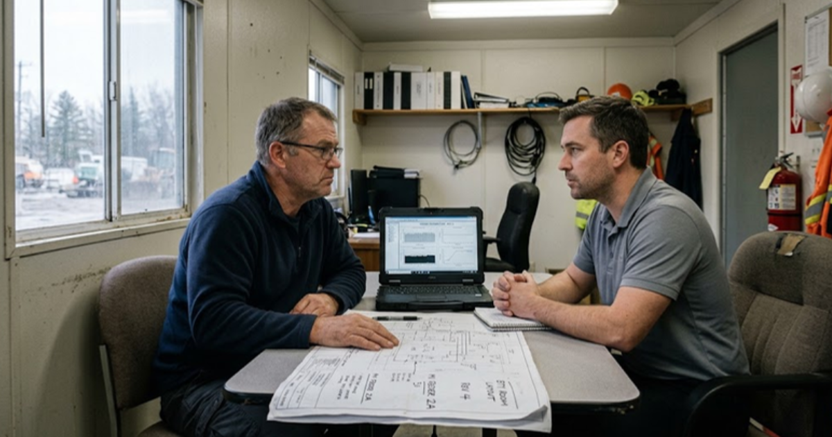
Interconnection studies fail when they describe the campus as one well-behaved block. The assumptions that break concern uniformity, voltage sensitivity, and how fast the load moves. Each one hides a behaviour that surfaces during the first serious fault.
- Treating the campus as constant power at all voltages, which hides the disconnection threshold.
- Assuming one ride-through setting sitewide when each hall shipped with different firmware.
- Modelling cooling as a fixed block instead of drives that respond to voltage.
- Using an annual average profile that erases the second by second steps a training cluster produces.
- Ignoring the harmonic current the rectifier front ends inject into the collector system.
Correcting these doesn’t require modelling every server. It requires protection settings hall by hall, the drive types in the mechanical plant, and an honest ramp profile from the orchestration team. Those three inputs move study results further than any refinement of the network model.
What accurate load models give planners and operators
Accurate load models give planners something they can act on. They show how much load stays connected during a fault, how much steps off, and how quickly the remainder moves afterward. That turns a large connection request from a capacity argument into an engineering one.
The discipline behind that is unglamorous. It means collecting settings nobody wrote down, keeping the spread between halls instead of averaging it away, and revalidating each time a new hall energizes with different firmware. Teams that skip it find out what their facility does the first time a nearby fault clears in three cycles. That’s the work OPAL-RT supports, putting facility controls and grid models in one real-time loop so the behaviour is measured before the utility measures it for you.
Microgrid
09 / 19 / 2026
Hybrid AC-DC microgrid emulation with power hardware-in-the-loop
An examination of how hybrid AC-DC microgrid stability is set at the interlinking converter and why power hardware in the loop is required to test that boundary at full power.

Power Electronics
09 / 17 / 2026
BLDC motor control fundamentals with simulation examples
A technical primer on six step BLDC commutation, Hall sensor and sensorless back EMF position sensing, torque ripple at each switching instant, and the simulation exercises a teaching lab can run.

Power Systems
09 / 16 / 2026
How to build a protection relay testing workflow utility engineers trust
A practical look at how utility engineers build protection relay testing workflows, from secondary injection through closed loop validation against a real time power system model.