Key Takeaways
- C-HIL judges a control law only as accurately as the I/O layer feeding it, so analog ranges, scaling and conditioning deserve verification before any firmware verdict is trusted.
- Sensor emulation is where most of the test value sits, because injected drift, quantization, noise and open circuits reproduce failure modes a physical rig cannot create safely or repeatedly.
- Signal level rigs answer control questions at low cost, and a power interface only becomes necessary once the question shifts to component behaviour under actual current.
Controller hardware-in-the-loop testing succeeds or fails at the signal layer, where a production embedded controller reads emulated sensor voltages and writes its commands back into a simulated plant.
Get the ranges, scaling and conditioning right and the controller can’t tell the difference between the simulator and the machine it will command. Get them wrong and you validate a cable loom instead of a control law. Faults that slip past the bench don’t stay in the lab. Safety recalls filed with the United States road safety regulator during 2025 covered 31.2 million vehicles across 997 campaigns.
CHIL puts a physical controller in a closed loop with a plant model running in real time, exchanging low-voltage signals rather than electrical power. Everything the controller believes about the machine arrives through a connector, so signal fidelity is the whole test. You’re checking firmware, timing, scaling and fault handling against a plant you can push into conditions no physical rig would survive.
What controller hardware in the loop actually tests
Controller hardware in the loop, written as C-HIL, tests a physical embedded controller against a plant model executing in real time. The controller runs its production firmware and sees emulated sensor signals on its input pins. Its outputs feed back into the model, closing the loop at signal levels rather than power levels.
A traction inverter controller on a C-HIL rig receives emulated phase current feedback, a resolver position signal and a DC link voltage reading, all synthesized from a motor model updating every few microseconds. Its six gate pulses return as digital captures on the FPGA, and the model answers inside the same timestep.
The scope is narrower and sharper than most teams expect. You aren’t proving the power stage works. You’re proving the control law computes the right answer from the measurements it will receive, with the resolution, latency and noise it will see. That boundary makes a failed test point at firmware rather than at hardware nobody has built.
How CHIL differs from power level HIL testing
The main difference between CHIL and PHIL testing is what crosses the interface. CHIL exchanges low-voltage measurement and command signals, so the equipment under test is the controller by itself. PHIL pushes actual current and voltage through an amplifier into physical apparatus, which makes the test much heavier to run.
Grid tied inverter programmes show the split. Firmware handling anti-islanding, ride-through and current regulation can be exercised on a signal-level rig, because every quantity it reads is a scaled voltage. Once the question becomes how the output filter heats under repeated fault current, the signal rig stops answering and a power interface is needed.
Most controller defects surface long before that point. Sequencing errors, saturation handling, ADC scaling mistakes and protection logic gaps live inside the firmware, and they show up the moment a model pushes the inputs to their limits. Teams that jump straight to a power interface spend weeks fixing bugs an inexpensive signal rig catches in an afternoon.
Signal levels and I/O ranges that carry controller interfaces
Signal level CHIL runs on a small set of standard electrical ranges. Analog outputs commonly span roughly plus or minus 16 V at 16-bit resolution, analog inputs accept plus or minus 20 V, and digital lines operate at 3.3 V or 5 V logic. Matching those ranges to the controller’s front end is the first setup job.
| Interface signal class | What the simulator sends or reads | What goes wrong when it is set up badly |
| Analog feedback for phase currents and bus voltages | Scaled voltages inside a plus or minus 16 V window, refreshed each timestep | Clipped readings make the controller act on a state that never occurred |
| Position and speed feedback | Emulated resolver, encoder or Hall patterns generated on the FPGA | Angle error shifts commutation and hides torque ripple |
| Gate commands leaving the controller | Digital pulses captured at nanosecond resolution and fed to the model | Coarse capture averages away the dead time that sets distortion |
| Discrete status and trip lines | Logic level lines at 3.3 V or 5 V with matched isolation | Threshold mismatch leaves protection paths untested until commissioning |
| Serial traffic on CAN or Modbus | Bus frames exchanged alongside the analog and digital channels | Timing skew against analog feedback produces faults you can’t reproduce |
Range headroom deserves more attention. A motor model peaking at 400 A of phase current, scaled through a 5 mV per amp sensor gain, needs 2 V at nominal and far more during a short circuit. Pick the scaling for nominal operation and every fault case saturates the channel silently.
Sensor emulation gives the controller the signals it expects
Sensor emulation converts model states into the electrical form each transducer would produce. A current sensor becomes a scaled voltage with the correct gain and offset. A resolver becomes a pair of modulated sine and cosine windings. The controller’s own conditioning circuit and ADC then do their normal work on that signal.
Fidelity at this layer matters. A study of 47 documented aerospace software failures found that unanticipated or erroneous sensor input accounted for 15% of cases. Defects of that shape only appear once a controller is fed signals its designers never planned for, which is exactly what an emulated sensor lets you do.
Good emulation includes the imperfections. Add the offset drift a Hall sensor shows as it warms, the quantization steps of the real ADC, the phase lag of the anti-aliasing filter and the open circuit of a broken connector. A controller that rides through those on the rig will ride through them in service, and each injection takes seconds.
“Defects of that shape only appear once a controller is fed signals its designers never planned for, which is exactly what an emulated sensor lets you do.”
Wiring an embedded controller into the closed loop
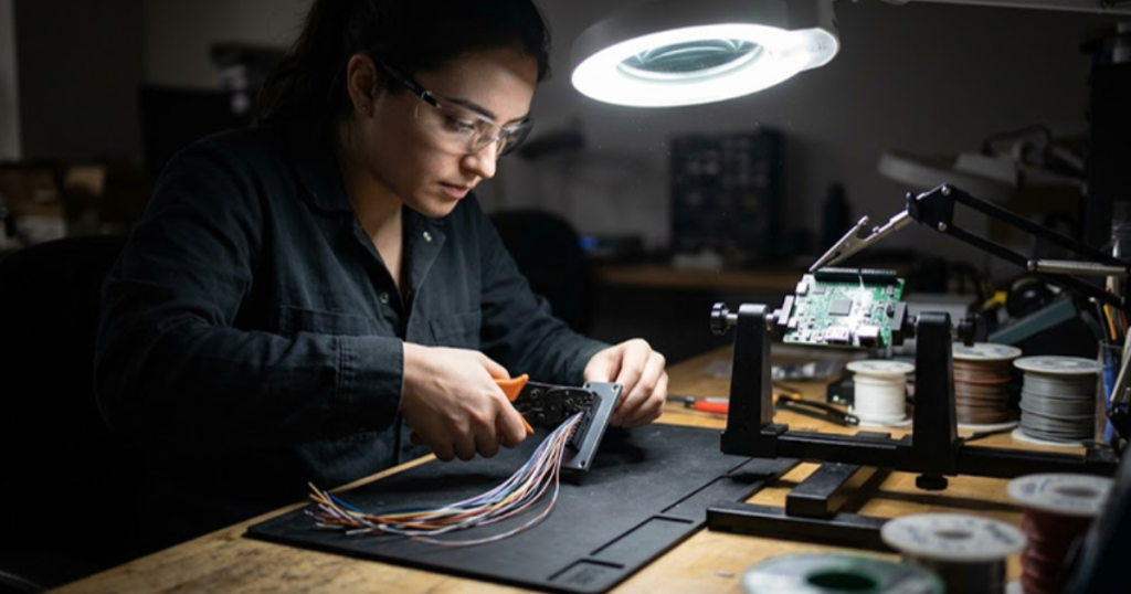
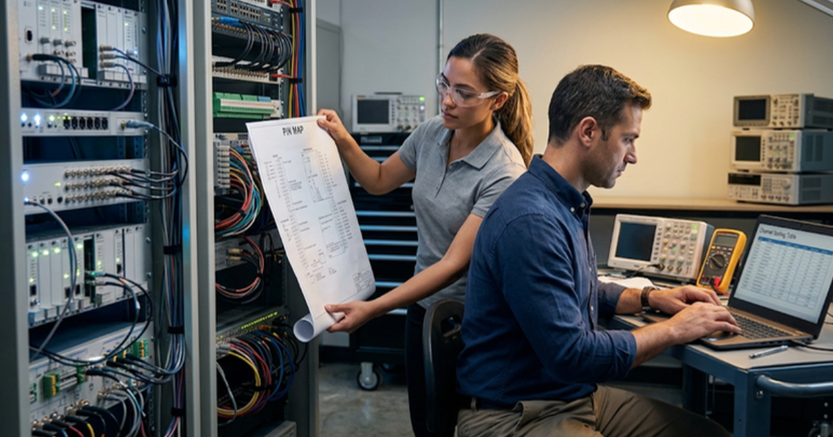
Connecting a controller to a CHIL rig means mapping every relevant pin to a simulator channel, then proving that mapping end to end before any control law gets judged. Scaling, grounding, isolation and update rates all get verified with the plant model held in a known steady state.
Five checks settle most setup problems teams hit on day one.
- Confirm each analog channel’s gain and offset by driving a known model value and reading it at the ADC.
- Verify polarity and phase order before closing the loop, since a swapped pair reads like an unstable control law.
- Match logic thresholds and isolation between the simulator I/O and the controller’s interface board.
- Measure end to end latency from model output to controller reaction, then represent it inside the model.
- Exercise every trip line while the plant sits in steady state, so protection paths get proven on their own.
Teams running RT-LAB on an OP5707XG keep signal conditioning and channel scaling inside the same configuration that holds the plant model, so the pin map and the physics stay in step when either one gets revised. That habit removes the most common source of wasted test days, a model edit that quietly invalidates a scaling constant.
Common signal level mistakes that invalidate CHIL results
Most invalid CHIL results trace back to four habits. Testing only at nominal operating points, ignoring the delay added by conditioning circuits, feeding the controller perfect signals, and leaving grounding or isolation unverified.
Perfect signals cause the quietest failures. A model handing the controller noiseless, infinitely resolved current feedback lets a marginal observer or filter design pass, and that design then oscillates the first time it meets a sensor carrying 8 mV of ripple. Adding measured noise back into the emulated channel costs nothing and changes what the test proves.
Latency is the other silent one. Signal conditioning, the ADC conversion window and the controller’s task scheduling each add microseconds, and a rig that doesn’t account for them reports a phase margin the deployed system won’t have. Measure the delay once with a step injection, put it in the model, and every stability result afterwards means something. Skipping it doesn’t give an obviously wrong answer, which is what makes it dangerous.
Building signal fidelity into every controller validation cycle
Signal level discipline pays off cumulatively rather than dramatically. Teams that verify scaling, latency and sensor realism at the start of a programme keep finding defects at the cheapest possible moment for years.
What separates a useful CHIL practice from a decorative one is the willingness to treat the I/O layer as engineering work in its own right, with its own documentation, regression checks and owner. That’s unglamorous next to the control algorithms it serves, and it’s the reason some labs catch a saturation bug in week two while others meet it during commissioning. OPAL-RT builds its controller interfaces around that assumption, giving signal conditioning and I/O range the same standing as the model that drives them.
Start with one controller, prove its interface honestly, and let the next programme reuse the pin map and the scaling records. Confidence in a control law is never stronger than confidence in the signals it was measured against.
“Confidence in a control law is never stronger than confidence in the signals it was measured against.”
Automotive
10 / 21 / 2026
Megawatt charging system validation for heavy duty trucks
A practical look at how the megawatt charging system works, how it differs from CCS and how charger controls are tested before a truck site is energized.
Automotive
10 / 19 / 2026
Dynamometer testing and motor emulation compared for e-drive programs
A comparison of dynamometer testing and motor emulation for e-drive programs, covering what each method proves, what it costs and how teams sequence both.

Power Electronics
10 / 17 / 2026
How wide bandgap devices push converter power density
Wide bandgap devices raise converter power density through faster switching and smaller passives, and this guide traces that chain from device physics to thermal limits to validation.