
Key Takeaways
- Start PHIL amplifier selection with closed-loop stability and total delay, because nameplate power does not predict loop quality.
- Four-quadrant behaviour, output impedance, and protection settings often decide test accuracy before amplifier class does.
- A solid-state power amplifier should only be narrowed to class A, class AB, or class D after the interface envelope is fully defined.
Choose a PHIL power amplifier from the loop back to the nameplate, because stability, delay, and four-quadrant behaviour will decide test quality long before watts do.
Teams often start with kilovolt-amperes and current peaks, yet PHIL breaks when the closed loop breaks. Published PHIL studies report loop delays from under 10 microseconds to beyond 100 microseconds across common laboratory setups. That range matters because an amplifier with strong brochure numbers can still add enough lag to disturb a converter or protection test. Your first filter should be loop behaviour, then electrical rating, then amplifier class.
That order answers the usual question about what amplifier is needed for PHIL. You need a power amplifier that can reproduce the interface signal with low and predictable delay, source and sink power in all required operating states, hold output impedance within the interface method’s tolerance, and survive faults without masking them. Once those conditions are met, class A, class AB, class D, and other solid-state power amplifier options become much easier to judge. You stop guessing and start matching the amplifier to the job.
“Strong power ratings will still fail you if delay, output filtering, or output impedance erodes phase margin and turns a stable model into an oscillating test.”
PHIL amplifier selection starts with loop stability limits
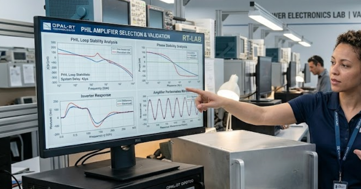
PHIL amplifier selection starts with loop stability because the amplifier sits inside the closed loop and directly shapes its behaviour. Strong power ratings will still fail you if delay, output filtering, or output impedance erodes phase margin and turns a stable model into an oscillating test. That is the first technical screen that matters.
A grid-forming inverter test shows the issue quickly. The simulated grid, interface algorithm, sensors, and power amplifier all sit in one feedback path, so a slight phase lag at a few kilohertz can turn a clean current response into ringing. If you’re only checking voltage and current ratings, you’ll miss the actual failure point. That kind of miss is common when a lab treats the amplifier like a generic source.
Selection should start with the interface method and the expected crossover region. Ideal transformer, partial circuit duplication, and damping-based interfaces each tolerate different amplifier traits. You want a unit whose small-signal behaviour stays predictable near the frequencies that matter to your loop. Bench performance at 50 or 60 hertz tells only a small part of the story.
Delay budget sets the usable bandwidth window
Delay budget sets the usable bandwidth because every microsecond between simulator output and measured feedback consumes phase margin. A PHIL amplifier with a flat frequency response can still behave poorly if transport delay, internal control delay, and measurement delay add up beyond what your interface algorithm can tolerate. Low delay that stays consistent matters more than headline bandwidth.
A converter control bench makes the delay chain visible. The simulator computes the plant, analogue output stages send the command, the power amplifier reproduces it, sensors return the response, and analogue input stages feed the loop. Teams using OPAL-RT often budget each step first, because a fast amplifier can’t rescue slow I/O or filtering upstream. That simple check keeps timing problems from being blamed on the wrong box.
Your usable bandwidth will sit well below the frequency where cumulative delay burns phase margin. That limit also affects amplifier class choice. A switched design with excellent efficiency can still struggle if output filters or digital control add enough lag near loop crossover, while a linear unit with less delay can stay cleaner over the required band. Delay is not a side note in PHIL. It is a sizing constraint.
Interface ratings define the required voltage current envelope
Interface ratings define the amplifier you need because PHIL stresses voltage, current, crest factor, and short-term overload far more unevenly than a sine-wave bench test. The right power amplifier will cover steady-state values, transient peaks, and the load line created by your interface model across the full operating envelope. Average power alone will hide the hardest parts of the job.
A motor drive test might need moderate continuous current but sharp regenerative peaks when torque reverses. A battery emulator might hold modest average power while asking for steep current steps during contactor events. Those cases punish undersized transient current headroom long before average kilowatts become the issue. You will feel the mistake during the first event test, not during a calm steady-state run.
You also need to read ratings the same way your test will use them. Three-phase apparent power, per-phase current, direct current bus swing, and overload duration will matter more than one large total power number. If the amplifier only meets the target under narrow duty assumptions, you’re buying a spec sheet rather than usable headroom. Good rating work matches the envelope at the terminals.
Four-quadrant operation avoids bidirectional power mismatch
Four-quadrant operation is required whenever the hardware under test can source and sink power, because PHIL will exchange energy in both directions as states shift. An amplifier that only sources power will distort regenerative events, force protective clamping, or send energy into dump loads that alter the behaviour you meant to measure. Bidirectional power flow is often a hard requirement, not an upgrade.
An inverter tied to a motor or grid emulator makes this plain. During acceleration the amplifier may source current, yet the same setup will return energy during braking or fault recovery. If the amplifier cannot absorb that reverse flow cleanly, bus voltage rises and the loop stops representing the intended plant. That means your test data now includes bench behaviour that should never have been there.
Bidirectional capability also has a practical cost-effectiveness. Dissipative handling of returned energy turns long regenerative tests into a thermal problem, while regenerative handling can keep the bench stable over longer runs. You should confirm sink rating, sink duration, and control behaviour during reversals, because brochure language around four-quadrant operation can be looser than it sounds. A vague claim here will cost time later.
Output impedance can destabilize the PHIL interface
Output impedance matters because the PHIL interface assumes the amplifier behaves like a certain kind of source over a certain frequency range. If the actual output impedance rises, resonates, or shifts with load, the hardware sees a different network than the simulator intended and closed-loop error grows quickly. That mismatch can look like plant error when the amplifier is the true cause.
A voltage-type interface into a stiff converter is a common trap. The model expects a low-impedance source, but the amplifier’s output filter and control loop can add inductive behaviour at higher frequencies. Current steps then overshoot, voltage recovery slows, and compensation settings start carrying work that the amplifier should have handled itself. You can spend days tuning around that hidden trait and still get a weak result.
Manufacturers rarely present output impedance in the form PHIL users need, so you’ll often have to infer it from small-signal data, closed-loop bandwidth, filter topology, and load dependence. A bench test with a programmable step and a known passive load will reveal more than a nominal spec. That check saves time before you tune interface compensation around a hidden amplifier trait. It also helps separate amplifier limits from model limits.
| Checkpoint | What you should confirm before purchase | What you will see if it is missed |
|---|---|---|
| Loop stability | The amplifier must stay predictable near the crossover region used by your PHIL interface. | The bench will ring or oscillate even when power ratings look sufficient. |
| Delay budget | Total delay from simulator output to measured feedback must fit the phase margin available. | Bandwidth shrinks and compensation effort rises before useful testing starts. |
| Voltage and current envelope | Steady-state values and transient peaks must both fit the amplifier’s usable range. | Short events will clip or fold back even though average power seems safe. |
| Four-quadrant power flow | The amplifier must source and sink energy for the full duration of regenerative states. | Returned energy will push the bench away from the intended plant behaviour. |
| Output impedance | Source behaviour at the terminals must match the assumptions built into the interface method. | Current steps, recovery, and closed-loop error will drift away from the model. |
Amplifier class selection follows fidelity heat constraints
Amplifier class selection follows loop limits because each topology trades signal fidelity, heat, size, and internal delay in a different way. Most PHIL benches use a solid-state power amplifier, then narrow the choice among linear stages such as class A or class AB, and switched stages such as class D. The class label only becomes useful after the loop is defined.
Thermal physics sets the first boundary. Open textbook calculations place ideal class A efficiency at 25% with a resistive load and ideal class B at 78.5%, which frames why linear designs run hot as power rises. A class a power amplifier can offer excellent small-signal behaviour, but it becomes hard to justify for higher-power PHIL unless fidelity at modest bandwidth matters more than heat and operating cost.
A class AB power amplifier usually gives the most balanced linear option, with lower crossover distortion than simple class B and less heat than class A. A class D power amplifier will deliver better efficiency and higher power density, yet its switching stage, filters, and control delay need closer scrutiny in PHIL. The right answer follows loop behaviour and thermal limits more than class labels. That is why a neat class chart won’t choose the unit for you.
Protection settings must not hide fault behaviour
Protection settings must support the test without rewriting it, because PHIL often studies the same abnormal states that protective firmware tries to suppress. Current limiting, foldback, overvoltage clamps, and latch-off thresholds should stay coordinated with the test plan so the amplifier survives faults while still showing the hardware’s actual response. Safe operation and honest data have to coexist.
A fault ride-through test shows the issue. The hardware under test may briefly pull far more current than its steady-state value, and a protective limit inside the amplifier can flatten that current before the device under test reaches its own control or protection threshold. You’ll think the hardware passed, yet the bench has silently changed the event. That error is subtle, and it is easy to miss during a busy commissioning week.
Protection review should cover timing as well as thresholds. Fast electronic current limiting can clip waveforms within microseconds, while slower thermal models act over seconds or minutes. You want visibility into both layers, plus clear logs that show when the amplifier entered a protected state. Hidden intervention ruins correlation between simulation, hardware traces, and later debugging. Good protection settings preserve the test while still protecting the rack.
A short selection workflow turns specs into a PHIL fit
A short selection workflow turns PHIL amplifier choice into a disciplined fit. Start with interface stability, assign a delay budget, map the voltage and current envelope, confirm four-quadrant power flow, and then compare classes and protections against the actual test duty rather than general lab preferences. That sequence removes the most expensive mistakes first.
“Good PHIL work comes from honest loop behaviour, and the amplifier has to earn that trust.”
A bench for a regenerative motor drive can look fully sized on paper, yet it’s still wrong on sink power, output impedance, or foldback behaviour. Each selection step removes a different failure mode before money is spent. A short pre-purchase review should answer these points clearly. Teams that skip this pass usually pay for it during integration.
- The interface method and loop crossover that the amplifier must support.
- The full delay budget from simulator output to measured feedback.
- The continuous and transient voltage and current envelope in each quadrant.
- The small-signal source behaviour the hardware must see at the terminals.
- The protection actions that are acceptable during faults and reversals.
Teams that keep this discipline get cleaner correlation, shorter commissioning, and fewer surprises during high-stress tests. OPAL-RT users often see the payoff when amplifier traits are matched to simulator timing before the first hardware hookup. Careful selection will spare you weeks of compensation tuning that was never going to fix a mismatched power stage. Good PHIL work comes from honest loop behaviour, and the amplifier has to earn that trust.
Real-time solutions across every sector
Explore how OPAL-RT is transforming the world’s most advanced sectors.

Industry applications
06 / 29 / 2026
What IEEE 2030.5 means for DER communication and dispatch interoperability
A practical guide to IEEE 2030.5, DERMS communication flow, protocol choice, device scope, testing, and tariff-led utility adoption.

Simulation
06 / 28 / 2026
How defense labs scale validation with real-time simulation platforms
This guide explains how defence labs use real-time simulation, HIL testing, and reusable models to validate vehicles and robotics before field trials.

Simulation
06 / 27 / 2026
Wind turbine simulation and testing for grid compliance engineers
This piece explains how engineers use wind turbine simulation, EMT studies, hardware-in-the-loop testing, and traceable metrics to support grid compliance work.