
Key Takeaways
- Closed loop stability is the condition that makes any PHIL accuracy claim believable.
- Delay, bandwidth, interface choice, amplifier dynamics, and controller gain must be checked as one loop.
- A stable margin measured on the bench gives you far more confidence than clean plots alone.
Closed loop stability determines if a PHIL result is trustworthy.
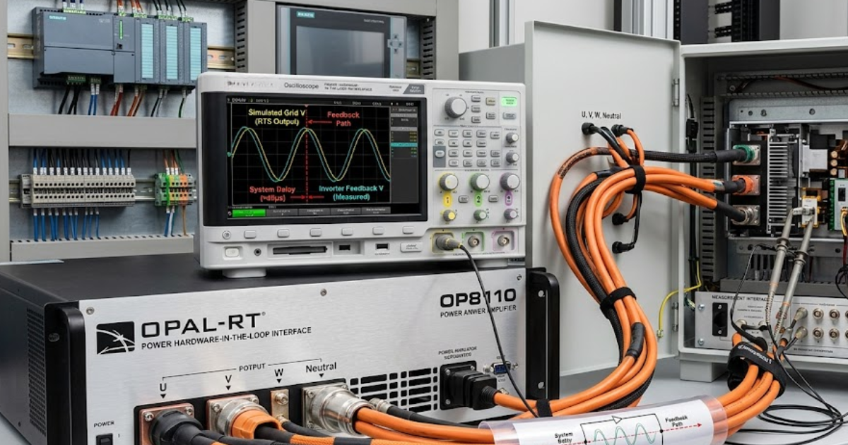
PHIL joins a simulated network to physical hardware, so every microsecond of delay and every gain choice feeds back into the same power exchange loop. Converter-heavy systems now make that judgement more important, and renewable electricity additions reached 507 GW in 2023, with solar accounting for 75% of that growth. You can’t treat accuracy as a later check. If the loop is unstable or close to unstable, the measured response will drift, ring, or look clean only because the test missed the frequencies that expose the problem.
“You need to check the stability of the closed loop as one system, because PHIL accuracy is a loop property.”
PHIL accuracy depends on stable power exchange loops
PHIL accuracy comes from a stable exchange of voltage, current, and power across the full loop. That loop includes the simulator, I/O, power amplifier, hardware under test, sensors, and interface model. Closed-loop stability keeps those parts aligned in time and magnitude. Once that alignment slips, accuracy goes first.
A grid-forming inverter connected to a simulated feeder shows this clearly. If the feeder model sends a voltage reference and the hardware returns current with extra lag, the loop starts to add energy at the wrong instant. You’ll still see sensible RMS values for a short period. The waveform shape, damping, and transient settling will already be wrong.
That is why closed-loop system stability matters more than any single device specification. A fast simulator won’t rescue a poor interface model, and a clean amplifier won’t rescue bad timing. You need to check the stability of the closed loop as one system, because PHIL accuracy is a loop property. Labs that separate component checks from loop checks usually miss the error until hardware power rises.
Delay creates phase error before tests look inaccurate
Delay is usually the first reason a PHIL setup loses trust. Every transport step, sensor filter, and amplifier response adds phase lag. That lag reduces the stability margin long before the test looks obviously unstable. A setup can pass a steady-state check and still fail during a transient.
A pure 100 µs delay adds 36° of phase lag at 1 kHz, which is enough to erase much of a comfortable phase margin. A battery inverter test makes that easy to see. Current tracking can look fine at low frequency, then overshoot sharply during a load step because delay shifted the crossover into a weak damping zone. What appears to be controller trouble is often simple loop latency.
You should treat delay as part of the plant, not as a small implementation detail. That changes how you estimate stability of a closed-loop system and how you choose bandwidth. Time delay compensation helps, yet compensation also depends on an accurate delay model. If you ignore delay during design and only notice it during energisation, you’re already tuning against a distorted loop
Bandwidth sets the ceiling for usable PHIL fidelity
Bandwidth defines the highest frequency range where the PHIL loop still behaves like the system you meant to test. When loop bandwidth sits too close to amplifier limits or I/O delay, fidelity drops before outright instability appears. You’ll get a result, but it won’t represent the intended physics.
A motor drive test bench shows the tradeoff well. If the hardware controller acts strongly up to 2 kHz but the amplifier and measurement chain remain clean only to a few hundred hertz, the loop will smear switching side effects and soften resonances. Current still flows, and protection logic still trips. The test still misses the timing and damping that decide if the controller is actually robust.
You should set usable bandwidth from the slowest high-impact element in the loop, then leave margin. That often feels conservative, yet it protects accuracy. Teams that chase wide bandwidth without checking phase and gain margins usually get attractive plots with poor meaning. PHIL does not reward nominal speed alone. It rewards a loop that stays controlled over the frequencies that matter for your test objective.
Interface models decide how much damping remains
Interface models shape the energy exchange between simulation and hardware, so they directly influence damping and stability. A mathematically neat interface can still behave badly when source stiffness and delay interact. Closed-loop stability depends on the interface choice because the interface changes the loop you are trying to control.
A stiff voltage source interface gives a simple setup for an inverter test, yet it can remove the damping that a physical feeder would provide. The loop then reacts as if the hardware is tied to an ideal source through delay. Oscillation appears near crossover, especially during sudden current reversal. A damping impedance or partial duplication approach often softens that behaviour enough to recover usable margins.
This is where many teams misread accuracy loss as hardware weakness. The hardware may be behaving correctly against a poor interface assumption. You should judge interface models by how they preserve passivity and damping under expected operating points. Once you do that, the stability of closed-loop system behaviour becomes easier to predict, and your test results stop drifting when operating conditions shift.
Power amplifier dynamics reshape the closed-loop response
Power amplifiers do more than scale voltage and current. They add delay, saturation limits, output impedance effects, and finite slew behaviour to the PHIL loop. Those dynamics reshape crossover and damping. If you model the amplifier as ideal, you will check the wrong loop and trust the wrong accuracy level.
A linear amplifier can offer smooth tracking at modest bandwidth, while a switched source can add control delay and filter behaviour that shifts resonance. That difference matters during a weak-grid inverter test. The same controller can look well damped on one bench and oscillatory on another because the amplifier changed the effective plant. On OPAL-RT platforms, engineers often separate solver delay, I/O delay, and amplifier delay before tuning, which makes the full loop easier to represent honestly.
| Loop element | What usually fails first | What you should verify |
| Transport delay in the loop | Oscillation begins near crossover even when steady-state values still look correct. | Total latency from solver output to measured feedback should be mapped and included in the loop model. |
| Limited amplifier bandwidth | Tracking lags at the frequencies where your controller still acts strongly. | Small-signal frequency response should stay clean over the useful test band with margin left over. |
| Interface model stiffness | The loop loses damping during fast current or voltage reversals. | Source and load assumptions should reflect the physical impedance you want the hardware to feel. |
| Excessive controller gain | Transient overshoot grows before obvious instability shows up. | Gain choices should be checked against the full PHIL loop, not a software-only plant. |
| Sensor filtering and scaling | Phase lag hides inside clean-looking measurements and corrupts fast events. | Filter delay and scaling should be measured under operating conditions, not assumed from datasheets. |
You should treat the amplifier as an active part of the stability problem. Bench measurements matter here more than nominal specifications. Small differences in output filter tuning or current limit behaviour can move the safe operating range enough to alter your findings. Once amplifier dynamics are included, PHIL accuracy becomes much easier to defend.
Controller gain sets the safe range for stability

Controller gain determines how aggressively the loop reacts to error, so it sets the safe operating window for PHIL. If you need to find the range of k for closed-loop stability, you must include delay, amplifier behaviour, and interface dynamics. A k value that works in software will often fail on hardware.
Consider a current controller with proportional gain k. A software-only model might support k from 0 to 1.8 before ringing becomes severe. Add amplifier delay and sensor lag, and the safe range can shrink sharply because the same gain now pushes crossover into poor phase margin. You’re no longer checking a controller in isolation. You’re checking the stability of the closed loop that PHIL actually creates.
That is why gain tuning should follow loop identification, not precede it. Start with a measured delay budget, then estimate crossover and margin, then move k upward in small steps while watching transient decay and spectral peaks. If you skip that order, k becomes a guess. Once you include the full loop, the stability of the closed-loop system behaviour becomes a design variable you can manage instead of a surprise you chase.
“If you need to find the range of k for closed-loop stability, you must include delay, amplifier behaviour, and interface dynamics.”
Stability checks must come before any accuracy claim
You can only claim PHIL accuracy after you verify that the closed loop remains stable over the operating points and frequencies that matter. Stability is the gate that every accuracy statement must pass through. If that gate is weak, even clean plots and repeatable runs won’t mean much.
A disciplined lab routine keeps the check simple and repeatable:
- Measure total loop delay under powered test conditions.
- Model amplifier and interface dynamics in the same loop.
- Confirm gain and phase margin near the intended crossover.
- Test transients that stress reversal, saturation, and weak damping.
- Reduce controller gain before widening bandwidth targets.
Those steps sound modest, yet they separate useful PHIL work from misleading PHIL work. A lab using OPAL-RT or any other real-time platform still has to earn accuracy through loop design and verification. Hardware speed helps, and open timing visibility helps, but neither replaces disciplined closed-loop checks. You’ll trust results more when each claim is tied to a measured margin and a known operating range.
The deeper lesson is simple. PHIL does not become accurate when the bench looks advanced or the plots look smooth. It becomes accurate when the loop remains stable under the same stresses your hardware will see during actual operation. That standard keeps your testing honest, and it keeps your engineering judgement grounded.
Real-time solutions across every sector
Explore how OPAL-RT is transforming the world’s most advanced sectors.

Power Systems
07 / 25 / 2026
Why distance protection relays mis-reach under real fault conditions
This piece explains why distance protection relays mis-reach under fault resistance, source infeed, capacitive voltage transformer transients, and heavy transfer, and how simulation-based testing checks zone reach before energization.

Power Systems
07 / 23 / 2026
Automating grid code compliance testing for inverter-based plants
Grid code compliance testing for inverter plants depends on weak grid studies, fixed disturbance definitions, repeatable scripted sequences, and structured pass/fail evidence.

Power Electronics
07 / 22 / 2026
Testing converter controls safely before connecting hardware
This page explains how fault injection, closed-loop plant models, and recovery checks help validate converter controls before hardware connection.